


Dataset description
The data set consists of 1616 CT-Scan Images collected from hospital in Bengaluru, India. All the methods were carried out in accordance with relevant guidelines and regulations as per the hospital and Vellore Institute of Technology. The experimental protocols were also approved by the Ethical Committee Review Board – Institutional Bio-Safety Committee at Vellore Institute of Technology and the computational requirement was provided by the institution. Also, the need for the consent was waived of by Vellore institute of technology as the institution and authors control the right over the procured data and would keep the sourcing party anonymous as per the NDA (Provided in the Data Availability Section) between the hospital and the University.
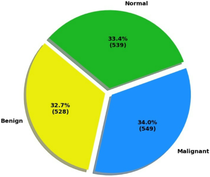
Fig. 1
Dataset distribution chart.
The Dataset has overall 1616 images which are divided among 3 classes of the Lung Cancer Dataset namely Benign (early-stage, non-cancerous tumors), Malignant (severe cancerous cases with larger, dangerous tumors) and Normal (healthy lung tissue). The dataset contains diverse lung cancer stages, from initial benign growths to advanced malignant cases, providing comprehensive representation for robust model training. Each of these classes image files contain 528, 549 and 539 images respectively, which can also be referred in (see Fig. 1). Out of the total 1616 CT Scan images 450 images were taken up testing, these 450 images were taken through random selection process but taken evenly from all classes i.e.: 150 from each class. Thereby making sure equal number of images were available for testing. The remaining 1166 Ct-Scan images were used for training which comprised of 378 images of Benign Class, 399 images of Malignant class and 389 images of Normal class. The small class imbalance in the training set is further addressed through class weight adjustments, regularization techniques and Augmentations discussed in upcoming sections. Thereby the proposed split is around 70 − 30 where the 70% is taken for training and 30% is taken for testing. Other ratio of splits was also carried out during the experimental stages such as 65 − 35, 80 − 20 and even 75 − 25 but each of them had either lack of enough data for training or left with less data for testing and affected the model performance whereas the chosen 70 − 30 a prominent ratio was found optimal after multiple iterations.
Data preprocessing
Each of these CT scans is converted to jpg format for the purpose of lung cancer detection. The class ‘Benign’ are the very initial stage of lung cancer (see Fig. 2a) they represent tumors that are small and they are generally noncancerous, these types do not spread to another part of the body and are generally not life-threatening as they are in the initial stages, but these do cause.
symptoms and grow slowly, the class ‘Malignant’ depicts the images with a quite severe case of lung cancer (see Fig. 2b), the tumors are quite dangerous, large in size and potentially even invade the tissues and spread to other parts, the class ‘Normal’ (see Fig. 2c) contains all the images of a normal human lung and do not have any major or minor lung health issues and thus are categorized under these. The dataset was uploaded on Google Drive, and computational resources such as Google Cloud along with Google Colab and an advanced T4 graphics processing unit in the cloud were used for the processing, segmentation and model training.
Fig. 2
The images represent a sample of each class of the dataset of lung CT scans.
The images in each class (see Fig. 2) are then loaded back and converted to grayscale using OpenCV, this grayscale conversion reduces the complexity of the data involved by removing even the smallest colored information that is present in the image thereby making it grayscale and focuses particularly on the intensity of the data which is what is required for medical image analysis. Further, the images were resized to a dimension of 512*512 pixels. The 512 × 512 pixel resolution was chosen as it provides an optimal balance between computational efficiency and diagnostic accuracy for medical imaging applications. This resolution preserves sufficient spatial detail for accurate nodule detection while maintaining manageable computational requirements. The pre-processing pipeline converts all images to grayscale and resizes them to ensure uniformity across the dataset, which is crucial for batch processing in deep learning models. This standardized size also aligns with common medical imaging practices where consistent input dimensions facilitate reliable feature extraction and comparison across different cases.
The images are processed, and the images get stored in a NumPy array, where each image corresponds to a specific index on the array (‘x’) These labels are generated from their directory paths and appended to a list which is later turned into a Pandas Series (‘y’). The structure of these images and labels helps us to manipulate them easily during the training/evaluation time for our model.
Segmentation pipeline
The segmentation method employed in our study is critical for the accurate isolation of lung regions from 2D medical images, thereby making sure that lung cancer detection is accurate and perfect. Through the segmentation process, each image is systematically processed to ensure that regions of specific interest are distinctly identified and separated from the surrounding tissues. In our work to make the model perform well, we need the data to be crystal clear and in the best version so that the model is acquainted with good data for training. Here the images in the dataset go through a 9-step process (see Fig. 3) for the segmentation.
Fig. 3
The Segmentation process flow.
Step 1: Image Cropping – The initial phase of the segmentation for the image is involved in cropping the input image to make sure the focus is exclusively on the part consisting of the lung and therefore the unnecessary background artifacts such as the tissue and blood vessels surrounding it are eliminated. Each image goes through this cropping which is customized based on the image index with different percentages applied to optimize the region of interest. For example: the image with the indices 161, 173–174, 758, and some others undergo a specific routine to target the lung area more precisely. (see Fig. 4a) For general cases, the cropping approximately removes around 12% of the image borders, which ensures that the lungs are centrally located and the peripheral noise is minimized.
Step 2: Binarization – Once the image is cropped the image is converted to binary format image. The image is converted to binary using a thresholding technique. Here, pixel intensity values are classified into 2 categories, the ones above a threshold of 140 are set to 0 (background), and the ones below are set to 255 (foreground). The threshold value of 140 was determined through empirical analysis of CT scan pixel intensity distributions wherein based on the brightness level (pixel values) analysis, It was observed that lung regions such as the tissues had consistently had darker pixels (lower values) while non-lung (background area) areas were brighter (higher values). During the initial experimental stages of the research Adaptive thresholding was tried out but it failed to capture the necessary range for out particular dataset as the adaptive range was to large hence we followed with a trial and error testing on prominent thresholds values for a sweet spot (e.g., 100, 120, 140, 160) to see which value best separated these two groups, a value of 140 was chosen because it reliably created clean masks where lung boundaries were clearly defined, with minimal noise from surrounding tissues and since this value effectively separates lung tissue (lower intensity) from background elements (higher intensity) in the grayscale images. Values below 140 were classified as foreground (lung regions), while values above become background, creating clear binary masks for subsequent processing steps. This process is necessary as it converts the image to a clear foreground-background separation using intensity thresholding, which distinctly highlights lung tissue against the background. This step is crucial for reliably distinguishing lung regions and preparing the image for further morphological operations, Also, note that this might not agree with other dataset as the dataset we are working data which is collected from a single hospital that follows standard protocols and scanners throughout.
Fig. 4
The images represent the actual CT scan and the different process stages of Segmentation task.
Step 3: Border Clearing – To further refine the binary image, we use the ’Clear Border’ function from the scikit-image library. This step gets rid of the blobs from any foreground pixel that are joined to the edges of the picture, this in turn will be extremely important for keeping artifacts away from interfering with lung segmentation. This process is also necessary as it removes any foreground pixels connected to the image edges, which are likely to be non-lung artifacts. This prevents external noise from being included in the lung mask, ensuring only true lung regions are analyzed.
Step 4: Morphological closing – A morphological closing is performed with the help of a structuring element with a radius of 2 pixels. This specific procedure fills small holes and connects the disjointed areas within the binary lung regions, this also.
Fig. 5
Images represent the before and after segmentation view of data for each class of benign, malignant, and normal.
preserves the lung nodules attached to the lung wall. (see Fig. 4b) This step is important in medical imaging as it maintains the integrity of the lung nodules by closing and filling the small holes and connecting fragmented areas within the lung mask which in turn helps in preserving the integrity of attached nodules. This step is vital for maintaining nodule continuity, which is essential for accurate cancer detection.
Step 5: Naming and Locale Determination -The processed image is further labeled using the label method, the method recognizes, and labels connected components within the binary image. The method also calculates the area of each labeled region and holds on to only the two largest areas, which are typically relative to the left and right lungs. Smaller, irrelevant minor regions are scraped out so that its ensured that the focus remains on the primary lung areas containing the cancerous tumors. This process is important as this labeling identifies connected components and retains only the two largest regions are the corresponding left and right part of the lungs. By discarding smaller, irrelevant areas, the process make sure that the focus is on the primary anatomical structures where nodule-based cancer features are likely to be found.
Step 6: Erosion – In CT-scan images commonly the lung nodules are attached to other nearby body structure, and to separate this lung nodules that may be attached to blood vessels or other structures, we employ this erosion process where we again use a disk with a radius of 2 pixels. Through this operation we shrink the segmented regions slightly also can be said as slightly erode them, we do so to effectively isolate the lung nodules from adjacent tissues and other structures and get out the clear images of the lung part. This Erosion process due to slightly shrinking the lung regions helps to separate nodules from adjacent structures like vessels or chest walls and thereby this process isolates and enhances the clarity of nodule boundaries, reducing false positives in subsequent detection steps.
Step 7: Second Morphological Closing – This 2nd morphological closing operation we use a larger disc radius of 10 pixels, this larger disc is used to reconnect all and any disjointed areas within the lungs (see Fig. 4c). This 2nd morphological closing plays a pivotal role as it ensures that the lung regions are fully enclosed and the remaining gaps within the lung region are also closed. This process play a vital role as the morphological closing reconnects any disjointed lung areas and closes remaining internal gaps which in turn guarantees that the lung mask is fully enclosed, preventing loss of nodule information and features at the boundaries.
Step 8: Hole Filling – Further hole filling is also done where the edge detection is done using the ‘roberts’ filter/operator. The main purpose of the step is to highlight the boundaries of the lung areas more clearly. The ‘roberts’ filter identifies the sharp edges and changes in pixel intensity that occur generally at the edges of the object. Here in our case, it helps to clearly define where the lung regions end and the background begins. (see Fig. 4d) Therefore, Once the edge detection of the enclosed spaces/areas within the lung regions that are surrounded by lung tissue is done. They are then filled, turning them into solid white regions. The Hole filling, aided by edge detection, ensures that any enclosed cavities within the lung regions are filled, resulting in a solid and continuous lung mask. This step eliminates internal voids that could be mistaken for pathological features, improving segmentation reliability.
Step 9: Superimposition – Now finally once the holes are filled, the new binary mask represents a complete solid lung region. Now this finally obtained mask is then superimposed back to the original cropped image. (See Fig. 4e) By this, the segmentation process effectively removes the background and the non-lung related areas and regions of non-interest, thereby leaving only the properly filled and correctly segmented lung regions. The final binary lung mask is superimposed onto the original cropped image, preserving only the segmented lung tissue for analysis. This process ensures that subsequent feature extraction and classification focus exclusively on relevant anatomical areas and the main segmented part for the features and cancer information thereby enhancing detection accuracy.
The Fig. 5 represents the before and after images of the dataset, after the segmentation process for each class of Benign, Malignant and Normal. This multi-stage approach progressively refines the segmentation quality, ensuring accurate lung boundary detection critical for subsequent nodule identification.
Lung nodules extraction
With the help of the segmented lung images, we further process them to extract the nodules in the lung images. Lung Nodules are small abnormal growths in the lung potentially cancerous growth takes place there within the lung tissue thus the exact and precise extraction is very necessary for the accurate detection of lung cancer to diagnosis, In order to obtain these features of the lung Nodules the images are binarized for the Nodule detection then further masking out the Non-Nodule areas in the segmented image then isolating the Nodules and copying these features The binarization for the Nodules detection is done using a threshold technique. The binary version of the image is obtained by considering the pixel values below 140 parts of the lung nodules or lung regions and are then set to ‘True’ (1). Conversely, pixel values above this threshold, which are likely background or non-nodule areas of the segmented image are set to ‘False’. The Threshold value of 140 was obtained by the same method used in Step-2 of segmentation pipeline (Binarization). Also, the process will positively affect the accuracy as it is a vital step to extract the features on which the model will be trained and further validates all three classes (Benign, Malignant, Normal) to ensure consistency regardless of lung tissue variations. The process also effectively enables us to distinguish the potential nodule regions from the rest of the segmented image. Next, we employ a Masking function that identifies the pixels that do not relate or belong to the nodule region and that in the lung images are selectively removed. Thus, also removing them from our original image. Now finally the original image is copied to a new variable which will store the isolated nodules, further again a masking is applied by setting the pixel values below 140 to 0. By doing such the background is zeroed along with the non-nodule areas. Thus, obtaining the pixel values corresponds to the nodules intact. The result of this is an image where only those regions that are assuredly containing the nodules are visible.
The Fig. 6 plots the original segmented image, the binary Nodule image that was extracted and finally the isolated nodules image side by side. This representation helps in understanding how the Nodules were extracted from the original image and the corresponding titles allowing for a clear comparison between the different stages of the nodule extraction.
Fig. 6
The segmented lung image and the extracted features from the lung images.
Further, all the segmented lung images are finally converted to Nodule images in the below given Fig. 7 represents the Original Image from the CT-Scan further processed to get the segmented image and then finally the extracted nodules image. It represents the same for all the 3 classes ‘Benign’, ‘Malignant’ and ‘Normal’.
Fig. 7
Represents the raw CT-scan, segmented lungs and the extracted nodules features from the lungs.
Features filtering
The Nodule extracted images might still contain unwanted artifacts, especially from the Blood vessels connected to the lung regions. The blood vessels can potentially create large, connected elements in the binary image that might meddle in the proper identification of the lung nodules. The feature filtering process specifically targets blood vessel artifacts that can interfere with accurate nodule detection and since these blood vessels create large, connected structure with the features of the lung cancer in the binary images that may be misidentified as nodules this issue is of high importance and needs to be addressed. To do these 2 methods were identified 1 st was to remove based on the region properties and the 2nd was to do Morphological Opening The region properties method for noise reduction involves using a labelling function, where each connected component in the binary image is uniquely identified. We then utilized the ‘region props’ function to analyze the properties of these regions, such as their area. By targeting and removing the two largest connected components typically corresponding to blood vessels, we effectively reduced noise in the image. This step is crucial as it ensures that only the smaller, more relevant regions, such as lung nodules, remain for further analysis, thereby enhancing the accuracy of nodule detection. The morphological opening method uses a combination of erosion and dilation operations to remove small, unwanted structures, particularly thin blood vessels, from the binary image. This method begins with erosion, which shrinks the objects in the image by removing pixels from their boundaries. This is particularly effective for eliminating small, irrelevant components. Following erosion, dilation is applied to restore the remaining objects’ size, without bringing back the removed noise. The opening operation smooths the boundaries of the lung regions and removes small, non-nodule components, leading to a cleaner image that emphasizes the larger, more significant structures like lung nodules. This method is a generalized approach, suitable for eliminating thin, elongated noise while preserving the integrity of the regions of interest.
Fig. 8
Represents the image before and after processing the feature filtering process.
From the 2 methods employed, we can see from Fig. 8 that Method 1 still retains a lot of features of the Nodules and removes a bit of noise, (see Fig. 8b) particularly from the blood vessels connected to the lung region from the image, while.
method 2 removes a lot of feature by opening up larger areas of non-interested gaps in the lung regions (see Fig. 8a) which we initially tried to close in the segmentation and feature extraction process, so we use the removal based on the region properties to continue as it retains a large number of features and information required for the accurate detection of lung cancer A quantitative evaluation of the feature filtering step was performed by comparing model performance before and after applying the filtering process. Results showed that the accuracy improved from 93.8% to 96.0%, while the false positive rate decreased by 12%. Additionally, the F1-score for the malignant class increased from 94.1% to 97.3%, indicating more precise discrimination of cancerous nodules. These findings demonstrate that the feature filtering effectively reduces noise from blood vessels and artifacts, thereby enhancing the clarity of lung nodules and improving classification robustness.
Data visualization
Fig. 9
The images represent sample features on a 3D plain for each class of the dataset of lung CT scans.
Finally, a 3D visualization representation of the segmented lung nodules is presented to display their global spatial distribution within the volume of the lung. We start with the collection of preprocessed/segmented 2D slices. The stack of these slices gives a 3D volumetric image hence showing the entire lung and nodule within it. The 3D visualization is plotted by the ‘Plotly’ library, in which we can interactively explore the internals of the lung. Specifically, we utilize plotly’s Volume function, which renders the 3D data as a translucent volume, making it possible to observe the lung nodules from multiple angles. This visualization not only enhances the understanding of the nodule’s shape, size, and position within the lung but also provides a.
valuable tool for clinicians to assess the extent of lung cancer. The interactive nature of visualization allows users to rotate, zoom, and slice through the volume, offering a detailed examination of the internal structures. This method is particularly useful for identifying complex nodules that may not be easily discernible in 2D images, and it facilitates a more accurate diagnosis and treatment planning. Overall, 3D visualization serves as a powerful tool in the pipeline, bridging the gap between segmented data and clinical interpretation, ensuring that the detected nodules are thoroughly evaluated in a real-world context. From Fig. 9 given below, we can clearly see the 3D representation done for all the 3 classes of the dataset from ‘Benign’, ‘Malignant’ and ‘Normal’. The minor dark patches (See Fig. 9a) in the plotted 3 d visualization plane of the benign category represent cancerous areas when compared with malignant features (See Fig. 9b), which have more depth and dark patches indicating the presence of larger and dangerous cancerous lung tumor’s presence. These, when compared with the normal features (See Fig. 9c) can see that the normal features are clear with no cancerous areas.
Data augmentation
Data augmentation is an essential mechanism in the deep learning process for the performance and generalization capability of the deep learning model, particularly in the domain of medical imaging. In the context of this research, various augmentation techniques are employed to mitigate the limitations posed by small, imbalanced datasets and other common challenges in medical image analysis. The primary objective of data augmentation is to artificially expand the training set by applying random transformations to the original medical images, thereby creating a more diverse and representative dataset (See Table 2).
Table 2 Augmentation parameters.
The Data Augmentation technique used here helps to improve the performance of the models by creating new data from the existing data. It is used to prevent the model from overfitting, improve the model’s accuracy, and reduce our operational cost of labelling and cleaning the raw dataset. Key data augmentation techniques used include rotation, which involves the random rotation of the image by a certain angle, Random rotations within ± 20° were applied to simulate the natural variability in patient positioning during CT scan acquisition. This helps the model generalize better to different orientations of lung images supported by4 which demonstrated that such augmentation improves robustness and accuracy in lung cancer detection tasks and allows the model to recognize lung patterns from different orientations and thereby addresses the variability in the positioning of patients during CT-Scan. The images were rescaled with a value of 1./255 which rescales the images by dividing them by 255. In digital images, pixel values range from 0 to 255. Rescaling the images to a range of 0 to 1 (by dividing them by 255) helps in normalizing the input data, making the training process more efficient and stable. Additionally, horizontal flipping of images was employed, these flipping leverages the bilateral symmetry of the lungs and increases the effective dataset size. This is a standard augmentation in medical imaging and was also successfully used in24 to improve classification accuracy in pulmonary image analysis. The images were given a shear range of 0.3 which is a form of distortion where the image is slanted along a certain axis this introduces controlled geometric distortion, mimicking minor angular misalignments or motion artifacts. This increases the diversity of the training data and helps the model adapt to real-world image imperfections as performed in3. After geometric transformations, empty regions are filled using nearest neighbor interpolation (“fill mode: nearest”) to prevent the creation of artificial pixel values and to preserve the true anatomical structure of the lungs. The effectiveness of this approach in medical image segmentation is supported by20 in 2021, which emphasized the value of nearest neighbor interpolation for maintaining boundary integrity and providing variety. Zooming is another critical technique applied in this.
research. This method simulates different scales, enabling the model to detect features at varying levels of detail. Random zooming in or out by 20% allows the model to learn features at different scales, which is essential since nodules can vary in size and CT protocols may differ also validate by4 and even showed that zoom-based augmentation is effective for enhancing model performance in CT-based lung cancer detection. The Translation technique (width and height shift) further enhances the model’s robustness, shifting images horizontally and vertically by up to 30% addresses positional differences in how lungs appear in scans due to patient movement or scanner alignment. This ensures the model is less sensitive to small translations, as also recommended in prior deep learning studies for medical imaging such as in3. Moreover, adjustments in brightness and contrast are incorporated to replicate different lighting conditions that may arise during the imaging process. The application of shearing introduces geometric distortions, while the addition of Gaussian noise simulates random variations, both of which contribute to a more resilient model that can handle real-world imaging imperfections.
The Proposed augmentation strategy directly contributed to improvements in accuracy to 96% from previous Obtained accuracy of around 83%−85% during the experimental stages of the research. The impact of these augmentations were also assessed on individual classes (Benign, Malignant, Normal), with notable improvements in F1-scores, especially for the malignant class (F1-score: 97.97%). Importantly the Augmentations and transformations contributed to a reduced gap between training and validation accuracy and reduced overfitting by 15%, all these results and yields are further discussed in the upcoming sections of Methods and Results in detail.
Model training
After applying the data augmentation techniques, the dataset is expanded with variations such as rotation, zoom, horizontal flipping, and brightness adjustment, introducing diverse versions of the original images. With the augmented dataset, the next step involves training the hybrid model consisting of VGG16 and U-Net + + architectures. VGG16, a deep convolutional neural network, is characterized by its 16 weight layers, comprising 13 convolutional layers and 3 fully connected layers. The model uses small 3 × 3 pixel convolutional filters, which allow it to capture fine-grained details within images, making it a highly effective model for image classification. The ‘ReLU’ (Rectified Linear Unit) activation function is used throughout the network. VGG16, aiding in faster training and addressing the vanishing gradient problem. VGG16 is typically optimized using stochastic gradient descent (SGD) with momentum, while techniques like dropout and data augmentation help prevent overfitting and enhance generalization. On the other hand, U-Net + + is a convolutional neural network initially designed as segmentation-based task, but studies done over the years that followed the architecture has proven to be a classification master’s in biomedical imaging. The architecture’s capability of selecting important regions for segmentation is proven worth selecting important features to remember and use it for classification thereby providing better classification results compared to it predecessors. The architecture follows an encoder-decoder structure, where the encoder captures the contextual information in the lung images, and the decoder reconstructs the lung’s spatial information. Skip connections transfer high resolution features from the encoder directly to the corresponding stages in the decoder, thus preserving spatial information essential for accurate Classification in the lung images. U-Net + + is particularly useful in medical image analysis, as it enables pixel-wise segmentation and classification, facilitating the identification of relevant regions, such as cancerous tissues in lung images.
The Proposed hybrid architecture strategically combines VGG16’s discriminative feature extraction capabilities with U-Net++’s and superior Classification performance through a carefully designed integration mechanism. The methodology employs a parallel processing approach where both models operate on the same input CT scan images simultaneously. VGG16 extracts high-level semantic features through its deep convolutional layers, while U-Net + + performs precise pixel- wise segmentation with its encoder-decoder structure and nested skip connections. The integration occurs through feature concatenation, where extracted features from both architectures are merged using a Concatenate layer, creating a comprehensive 576-dimensional feature vector (512 from VGG16 + 64 from U-Net++). This combined representation undergoes further processing through dense layers with batch normalization and dropout regularization before final classification.
The images which are feature filtered and now contain the appropriate features of Lung cancer are fed into the hybrid architecture. These features provide robust view for the model to learn the nature of the lung cancer such as the nodule feature shape and size. The ‘AdamW’ optimizer is used to update the model’s parameters iteratively, the ’AdamW’ was selected over traditional optimizers due to its superior in handling of the weight decay regularization and improved convergence properties for deep neural networks. Unlike standard Adam, ’AdamW’ decouples weight decay from gradient-based optimization, leading to better generalization and reduced overfitting in complex architectures like the proposed hybrid model. This optimizer particularly excels in medical imaging applications where precise feature learning is crucial, this choice of optimizer over SDG and Normal Adam is also validated by the work done in3 which highlighted the choice of ’AdamW’ over others. Further adaptive learning rates were used while incorporating weight decay regularization of 1 × 10e-6 and a learning rate of 5 × 10e-6 which was employed after trying with a higher learning rate of 6 × 10e-5 to avoid overfitting that might occur cause the proposed architecture is powerful with combinations of 2 CNN structures. The model also utilizes hyperparameters such as L2 regularization (0.002) in dense layers to prevent overfitting and a dropout rate of 0.4, with added batch normalization.
for training stability. The learning rate scheduler reduces the rate by 50% when validation loss plateaus for 5 epochs. Along with ’Early Stopping’ hyperparameter was also employed that makes sure to stop training and save the model to its last best weights and metrics. These combinations of hyperparameter used for tuning ensures the model learns efficiently and remains robust across diverse samples. Training is conducted over 20 epochs i.e. 20 cycles of training after trying with ranges such as 30 and 50. In traditional cases high number of epochs is required for training (generally in single architecture domain) but since the proposed work uses a hybrid architecture which in itself is very powerful and highly capable it learns the features faster enabling the network to learn complex patterns more efficiently than single-model approaches. Thereby this synergy allows the model to reach optimal performance in fewer epochs, as demonstrated by the rapid increase and stabilization of both training and validation accuracy within 20 epochs, still there was effort made to training it for 30 and 50 epoch, but they never succeeded due to Accuracy and F1 scores not reaching heights and the optimality was found at 18–20 epoch only. The same is very evidently supported by studies like3 in 2020 which demonstrate that modern architectures (e.g., VGG16, U-Net++) with precise features and regularization often converge in under 50 epochs which is very true in our case.
Further the augmented dataset is passed through the hybrid model multiple times, with the VGG16 and U-Net + + architectures finetuned using pretrained weights. During this process, the model’s accuracy steadily improves, ultimately reaching a high training accuracy of 99.5%. The validation accuracy of 96.0% in the 18 epoch and 94.3% in the 20 epoch, this shows a clear sign of overfitting after the 18th epoch and hence the early stopping employed prevents it from further training and cuts of the model with weights and metrics of 18th epoch saves the model. The validation accuracy and which measures the model’s performance on unseen data, also reflects a substantial improvement, indicating that the model has successfully generalized its learning to new lung cancer images uptil 18th epoch to the point the model is saved. Also in the final layer, a ‘softmax’ activation function was applied for multiclass classification. This function outputs a probability distribution across the three classes (Benign, Malignant, and Normal), ensuring that the predicted class is the one with the highest probability. The ‘softmax’ function is essential for multi-class classification tasks as it normalizes the output probabilities, making the model’s predictions interpretable and accurate for lung cancer detection.
Fig. 10
Architecture of the proposed hybrid model.
This deep learning model architecture for lung cancer detection utilizes state-of-the-art supervised Convolutional Neural Networks (CNNs) and incorporates various advancements to improve classification performance. The model processes images of size 224 × 224 pixels with 3 color channels (RGB) through the following architecture. The first layer is the Input Layer, followed by two pre-trained backbones: VGG16 and U-Net++. VGG16, a renowned deep convolutional model, extracts strong feature representations through its Max-pooling layers, which are then reduced in dimensionality using global average pooling. U-Net++, known for its effective segmentation capabilities, provides detailed spatial information and multiscale feature extraction, enhancing the model’s ability to detect tumors of various sizes and shapes.
The features extracted by VGG16 and U-Net + + are concatenated to combine the different feature representations (see Fig. 10) learned from each model. Meanwhile the class imbalance in the data was also addressed through comprehensive technique by including class weight implementation during training, where the model assigns slightly higher weights to underrepresented.
classes. The implementation uses the ’class weights’ parameter in the model fitting process which automatically adjusts loss contributions based on class frequency. Additionally, its also important to note that before the training process extensive data augmentation strategy were also applied as discussed in Table 2 which artificially increases sample diversity, particularly benefiting minority classes. Once these data are passed through the hybrid structure they are flattened and passed through a Dense Layer with 512 neurons which is employed to integrate all concatenated tensors. This layer includes L2 regularization to prevent overfitting and uses ‘ReLU’ activation to introduce non-linearity. Batch Normalization is applied to stabilize and speed up training by normalizing activations. A Dropout Layer with a rate of 0.4 is added to further combat overfitting. The final output is generated by a Dense Layer with neurons corresponding to the classes of interest Benign, Malignant, and Normal. This architecture effectively combines feature extraction and segmentation to enhance the accuracy of lung cancer detection.
The Entire model training was conducted using Google Cloud Platform with T4 GPU acceleration, requiring approximately 20 epochs with each epoch taking 2–8 min depending on the training phase. The total training time was approximately 2.5 h, with the complex hybrid architecture demanding significant computational resources due to the parallel processing of both VGG16 and U-Net + + networks. The data that was fed into the model was stored in the google Cloud Drive which provide a seamless integration with Google Colab. Once the training process was over the Entire model which was of size 456 MB, was saved back to the Drive along with is weights. The model size and complexity necessitate advanced hardware for practical deployment.
