


Appendix A
Nomalization in Eq. (7) uses \(V_{obs}\) rather than \(V_0\)
Although the values of \(V_{obs}\), \(\alpha\) and \(\beta\) in MBBG equation depend on whether the experimental data are fitted starting from or after \(V_{obs}\), it can be shown that these three parameters are not independent and the solution function is always the same, as shown below.
The MBBG equation is given by
$$\begin{aligned} V(t)= V_{obs} \left( \frac{V_0}{V_{obs}}\right) ^{e^{-\beta t}} e^{\frac{\alpha }{\beta }(1-e^{-\beta t})}. \end{aligned}$$
(11)
If instead of using \(V_{obs}\), \(\alpha\) and \(\beta\) in MBBG equation, we use \(V_{obs}^* = rr V_{obs}\) and \(\alpha ^* = \alpha -\beta \ln (rr)\) for obtain
$$\begin{aligned} \begin{array}{rl} V^*(t)= & V_{obs}^* \left( \frac{V_0}{V_{obs}^*}\right) ^{e^{-\beta t}} e^{\frac{\alpha ^*}{\beta }(1-e^{-\beta t})} \\ = & V_{obs} \left( \frac{V_0}{V_{obs}}\right) ^{e^{-\beta t}} (rr)^{(1-e^{-\beta t})} e^{\frac{\alpha ^*}{\beta }(1-e^{-\beta t})} \\ = & V_{obs} \left( \frac{V_0}{V_{obs}}\right) ^{e^{-\beta t}} [(rr) e^{\frac{\alpha ^*}{\beta }}]^{(1-e^{-\beta t})} \\ = & V(t), \end{array} \end{aligned}$$
(12)
that is, the function is exactly the same. From biophysical point of view, this may mean that the growth of a unperturbed cancer type in a given host is unique, known as the natural history of cancer in preclinical13,14,30–32 and clinical41 studies. Therefore, in principle, either \(V_{obs}\) or a value greater than it (e.g., \(V_0\)) may be chosen interchangeably for normalization. In order to compare MBBG or Richards equations with the mKJMA function, we must take into account that the evolution in the case of mKJMA goes from \(t=0\) to \(t= \infty\), meaning that the unperturbed cancer initiates its growth at \(t=0\) until it reaches its maximum value 1 at \(t=\infty\), as in experiment13,14,30–32. In the case of MBBG or Richards equation, it goes from \(t= -\infty\), where the unperturbed cancer volume is zero, to \(t=\infty\) where the maximum value is reached. Normalizing MBBG, Richards to the interval \([0,\infty ]\) requires the selection of an instant \(t^*\) at which the unperturbed cancer volume \(V(t^*)\) is small enough to consider it the starting point of the tumor growth, so that the interval \([t^*,\infty ]\) contains the relevant evolution of the tumor and it can be transformed to the interval \([0,\infty ]\). For this, if we replace \(t+ t^*\) with t, the function \(q_i(t)\) is modified. Then, the normalized MBBG and Richards equations can be defined by
$$\begin{aligned} q_i(t) = \frac{V(t+ t^*)-V(t^*)}{V(\infty )-V(t^*)}=\frac{V(t)- V^*}{V(\infty ) -V^*} + \frac{V(t+t^*)-V(t)}{V(\infty ) -V^*}, \end{aligned}$$
(13)
and since the derivate \(V'(t^*)\) will be small and the denominator can be large, the modification is small; therefore, it is better to use the function without approximation. Thus, \(q_i(0)=0\) for \(t=0\) and \(q_i(\infty )=1\) for \(t=\infty\), as in Avrami formulations13,16.
In Ref.16, the unperturbed cancer volume at \(t=0\) is small enough, and therefore taking \(t^*=0\) is reasonable. Nevertheless, in the present case, \(V(t= 0)= 0.5 cm^3\), the first measured volume in the experiment, which is too large and consequently, valuable unperturbed TGK information for \(V(t) < 0.5 cm^3\). Therefore, a more reasonable option in this case is to take \(t^*= t_{obs}\), such that \(V(t^*) = V(t_{obs}) = V_{obs}\) for two reasons: 1) Since \(V_{obs}\) is the smallest volume that can be estimated from experiment (\(V_{obs} < V_0\))14 and the interval \([t_{obs}, \infty ]\) contains most of the information about the evolution of the unperturbed cancer. Note that since \(t=0\) corresponds to the first measured volume \(V_0 = 0.5 cm^3\), then \(t_{obs}\) is necessarily negative, which means that the unperturbed cancer volume \(V_{obs}\) is attained \(t_{obs}\) units of time before the first time its volume is measured. 2) \(V_0\) depends on how the measures have been done, whereas \(V_{obs}\) is in fact the unperturbed cancer volume reached at the latency time, which is a characteristic time of each type of unperturbed cancer growing in a host. In conclusion, the normalized MBBG and Richards functions are defined by
$$\begin{aligned} q_i(t) = \frac{V(t+ t_{obs})-V_{obs}}{V(\infty )-V_{obs}}. \end{aligned}$$
(14)
This expression coincides exactly with Eq. (7) if the reference system in the unperturbed TGK is located at (\(t_{obs}\),\(V_{obs}\)).
Appendix B
Richards model and its connection with the Gompertz model
Considering that a generalized Gompertz function can be written as
$$\begin{aligned} y(t) = K \exp \!\left[ -b e^{-ct}\right] , \end{aligned}$$
(15)
and the Richards model as
$$\begin{aligned} y(t) = K\left[ 1 + m\, e^{-ct}\right] ^{-1/m}, \end{aligned}$$
(16)
where K is the carrying capacity, \(c\) is a growth parameter and \(m\) controls the asymmetry of the sigmoidal curve. Then, the Richards model may be connected with the Gompertz model by means of the following substitution \(z = 1 + m\, e^{-ct}\), which transforms the solution as \(y(t) = K z^{-1/m}\). Now, taking the logarithm, \(\ln y = \ln K – \frac{1}{m}\ln z\) and expanding for \(m\rightarrow 0\), we obtain \(\ln y \approx \ln K – \frac{1}{m} (m e^{-ct})\). Applying the exponential function to both sides and considering the limit, we obtain
$$\begin{aligned} \lim _{m \rightarrow 0} K\left( 1 + m e^{-ct}\right) ^{-1/m} = K \exp \!\left( -e^{-ct}\right) , \end{aligned}$$
(17)
which corresponds to the Gompertz growth model. This result shows that the Gompertz model can be interpreted as the singular limit \(m \rightarrow 0\) of the Richards model. Therefore, the parameter m controls the deviation from the Gompertz dynamics and determines the asymmetry of the sigmoidal growth curve.
Appendix C
Construction of a fractal complexity for MBBG mapping
The Gompertzian analysis of experimental tumor growth distinguishes successive dynamical regimes and reports interval-dependent temporal fractal exponents, denoted here by \(b_I\) and \(b_{II}\)40. The decrease from the first to the second regime was interpreted as a loss of dynamical complexity during tumor progression39. In that framework, the fractal exponent is not merely a curve-fitting parameter: it summarizes changes in temporal organization, effective connectivity, and the number of dynamically active degrees of freedom involved in the growth process.
Additionally, the MBBG formulation introduces a kinetic–geometric coupling in which the effective contour exponent \(d_f\), the mass fractal dimension \(D_f\), and the kinetic quantity \(u_2\) are related14,39. This provides a natural bridge between temporal multiscaling and spatial organization. Our working hypothesis is therefore that the transition from regime I to regime II leaves a measurable geometric signature. Accordingly, the decrease in temporal fractal complexity is used as a phenomenological proxy for progressive reorganization of the tumor interface and of the proliferative population.
This hypothesis is physiologically motivated by the fact that early tumor expansion is dominated by proliferation and collective organization, whereas later growth is increasingly affected by nutrient limitation, hypoxia, mechanical confinement, competition, heterogeneous viability, and loss of effective cell–cell connectivity. The difference between the temporal fractal exponents is thus interpreted as a coarse-grained measure of the magnitude of the dynamical transition, rather than as a direct measurement of a spatial fractal dimension. Here, we assume that the contour exponent responds to the absolute loss of temporal complexity, \(\Delta b_i=b_{I,i}-b_{II,i}\), through
$$\begin{aligned} d_{f,i}=c_0+c_1\Delta b_i. \end{aligned}$$
(18)
For each tumor, the Gompertzian parameters were mapped to the MBBG variables according to
$$\begin{aligned} \alpha _i=\kappa _i A_i, \qquad \beta _i=a_i, \end{aligned}$$
(19)
where \(A_i\) and \(a_i\) are the parameters of the original Gompertz representation and \(\kappa _i\) is the kinetic renormalization factor obtained in the preceding regularized mapping. The observable scale was restricted to the narrow interval \(0.15\le V_{\textrm{obs},i}\le 0.19\), consistent with the exploratory observable-volume range used in the MBBG analysis14. For a given candidate value of \(d_{f,i}\), the kinetic–geometric quantity or apoptosis velocity \(u_{2,i}\) was computed as
$$\begin{aligned} u_{2,i} = \frac{ \alpha _i+\beta _i\ln V_{\textrm{obs},i} }{ \ln \left[ \dfrac{\frac{2}{3}d_{f,i}-1}{d_{f,i}-1} \right] }, \end{aligned}$$
(20)
and the effective fractal dimension was obtained from
$$\begin{aligned} D_{f,i} = \frac{d_{f,i}}{1-\beta _i/u_{2,i}}. \end{aligned}$$
(21)
The admissible domain was restricted to positive \(u_{2,i}\) and the interval was used as a physical plausibility constraint for the present exploratory construction and should not be interpreted as an independently measured value for every tumor.
The coefficients \((c_0,c_1)\) of each candidate law were estimated by constrained numerical optimization. The exploratory objective function combined three elements: (i) proximity to the central geometric scale \(D_{f_0}=1.2\), (ii) a large penalty for solutions outside the admissible interval \(1.0\le D_f\le 1.4\), and (iii) a weak penalty against collapse of the between-tumor dispersion. In symbolic form,
$$\begin{aligned} \mathscr {J} = \frac{1}{N}\sum _{i=1}^{N}(D_{f,i}-D_{f_0})^2 + \lambda _C\mathscr {P}_{\textrm{phys}} + \lambda _S\mathscr {P}_{\textrm{s}}, \end{aligned}$$
(22)
where \(\mathscr {P}_{\textrm{phys}}\) penalizes violations of the physical interval and \(\mathscr {P}_{\textrm{s}}\) prevents a trivial constant-\(D_f\) solution. The contour exponent was additionally required to remain in the stable mathematical domain \(0.50. A leave-one-tumor-out procedure was then performed. At each iteration, the coefficients were re-estimated from the remaining tumors and the excluded tumor was evaluated with the resulting law. This procedure measures internal robustness of the constrained construction. It is not an external validation against independent measurements of spatial fractal dimension.
The temporal exponents \(b_I\) and \(b_{II}\) quantify the organization of growth fluctuations across successive dynamical regimes, whereas \(d_f\) and \(D_f\) describe effective geometric quantities within the MBBG framework. The relation of \(d_f\) does not assert that a temporal fractal exponent is identical to a spatial fractal dimension. Instead, it assumes that the magnitude of the temporal complexity loss contains information about the structural reorganization accompanying tumor progression.
The positive coefficient multiplying \(b_I-b_{II}\) implies that a larger dynamical transition is associated, within the present mapping, with a larger effective contour exponent. Physiologically, this can be read as the geometric imprint of a transition from a relatively coordinated proliferative regime toward a state increasingly shaped by heterogeneous constraints. These may include spatially uneven nutrient availability, hypoxia, necrotic development, mechanical stress, heterogeneous proliferative activity, and weakened effective connectivity among cell populations.
Analytical propagation of uncertainties
The reported uncertainties of the Gompertz parameters \((A,a,b_I,b_{II})\) were propagated through the MBBG mapping using first-order Gaussian error propagation. For \(d_f = c_0+c_1(b_I-b_{II})\), we obtain \(\sigma _{d_f}= \sqrt{\sigma _{c_0}^2+(b_I-b_{II})^2\sigma _{c_1}^2+c_1^2(\sigma _{b_I}^2+\sigma _{b_{II}}^2)}\). For \(\alpha =\kappa A\), \(\sigma _\alpha =\alpha \sqrt{\left( \frac{\sigma _\kappa }{\kappa }\right) ^2+\left( \frac{\sigma _A}{A}\right) ^2}\). \(\beta =\alpha ^*\), then \(\sigma _\beta =\sigma _{\alpha ^*}\). Define \(L=\ln \left( \frac{\frac{2}{3} d_f-1}{d_f-1}\right)\), with \(\sigma _L=\left| \frac{\frac{2}{3}}{\frac{2}{3}d_f-1} -\frac{1}{d_f-1} \right| \sigma _{d_f}\) and \(N=\alpha +\beta \ln (V_\textrm{obs})\), then \(\sigma _N= \sqrt{ \sigma _\alpha ^2 +(\ln V_\textrm{obs})^2\sigma _\beta ^2 +\left( \frac{\beta }{V_\textrm{obs}}\right) ^2\sigma _V^2}.\) The kinetic parameter is \(u_2=\frac{N}{L}\), with \(\sigma _{u_2} = u_2 \sqrt{\left( \frac{\sigma _N}{N}\right) ^2+\left( \frac{\sigma _L}{L}\right) ^2}\). Finally, \(D_f=\frac{d_f}{1-\beta /u_2}\). Defining \(Q=1-\frac{\beta }{u_2}\), its uncertainty is \(\sigma _Q= \sqrt{\left( \frac{\sigma _\beta }{u_2}\right) ^2+ \left( \frac{\beta }{u_2^2}\sigma _{u_2}\right) ^2}\), and \(\sigma _{D_f} =\sqrt{\left( \frac{\sigma _{d_f}}{Q}\right) ^2+ \left( \frac{d_f}{Q^2}\sigma _Q\right) ^2}\). These expressions provide a complete analytical propagation of uncertainty from the experimentally estimated Gompertz parameters to the inferred MBBG quantities.
Table 2 Tumor growth parameters and corresponding MBBG variables.
Appendix D
Construction of a fractal forbidden zones in mKJMA model
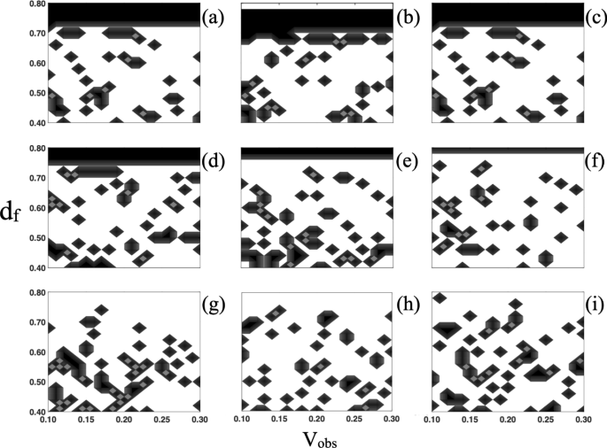
See Fig. 10.
Fig. 10
2D Contour maps, p(t) versus \(d_f\) and \(V_{obs}\) at \(t = 10\) days, for mKJMA model. The parameters values \(u_2 = 0.620\) days\(^{-1}\) and \(D_f \in [1.00, 1.40]\) with intervals of 0.05 from (a)-(i) panels, respectively. The black regions delimit forbidden zones of the parameter space, where the model mKJMA predicts no admissible tumor growth dynamics.
