


Ethics statement
All research complies with all relevant ethical regulations. Animal experiments were performed with the approval of the Institutional Animal Care and Use Committee of Tsinghua University (17-ZQF1.G23-1). Human CRC samples were collected and used with the approval of the Medical Research Ethics Committee of Beijing Chao-Yang Hospital, Capital Medical University, and written informed consent was obtained from all participants.
Cell culture
The human HEK293T (SCSP-502) and mouse NIH/3T3 (SCSP-515) cell lines were newly purchased from the Cell Bank of the Chinese Academy of Sciences. The identities of these cell lines were authenticated by the vendor before purchase, and they were routinely tested negative for Mycoplasma contamination. Neither line is listed in the International Cell Line Authentication Committee database of misidentified cell lines. HEK293T and NIH/3T3 cells were cultured in Dulbecco’s modified Eagle’s medium (DMEM) (C11995500BT, Thermo Fisher) supplemented with 10% fetal bovine serum (FBS) (P30-3302, PAN BIOTECH) at 37 °C with 5% CO2. Cells were rinsed with PBS (C10010500BT, Thermo Fisher) and detached by incubating for 3–5 min at 37 °C with 1 ml of 0.25% Trypsin-EDTA (25200114, Thermo Fisher). Detached HEK293T and NIH/3T3 cells suspensions were collected via centrifugation, washed with PBS and counted using a C-Chip Disposable Hemocytometer (DHC-N01N, As One).
Three-dimensional spheroids culture
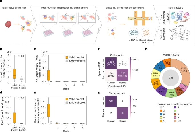
HEK293T and NIH/3T3 cells were cultured as mentioned above. AggreWellTM400 six-well microwell plates (34421, StemCell) were prepared following the manufacturer’s instructions. A total of 42,000 cells were seeded per well (approximately six cells per microwell) and cultured in the humidified incubator at 37 °C with 5% CO2 for 24 h. HEK293T and NIH/3T3 spheroids were carefully collected, and single cells were separated by passing through a 10-μm strainer. Approximately 20,000 spheroids per type were prepared and labeled with human- or mouse-specific indexed CMOs, followed by three rounds of split-pooling barcoding.
Mouse studies
Six WT C57BL/6J male mice (6–8 weeks) were purchased from the Laboratory Animal Research Center at Tsinghua University. Mice were housed in a specific-pathogen-free facility under a standard 12-h light–dark cycle. The ambient temperature was maintained at 20–24 °C, and the humidity was kept at 40–60%. Three Apcflox/flox; Villin-CreERT2 male mice64 (about 12 weeks old), kindly provided by Y.-G. Chen (Tsinghua University), were intraperitoneally injected with 200 µl of tamoxifen dissolved in sunflower oil at a concentration of 10 mg ml−1, and the small intestine was isolated 7 days later for CCI-seq or tissue fixation.
Clump isolation from mouse kidney
Kidneys from WT C57BL/6J mice were collected and transferred to a 1.5-ml EP tube. We added 1 ml of dissociation solution (4.8 mg ml−1 Dispase II, 3 mg ml−1 Collagenase IV, 0.1 mg ml−1 DNase I and 10 mM CaCl2 in PBS) and used scissors to repeatedly mince the tissue on ice for about 2 min until most of the tissue fragments were approximately 1 mm in size. Then, we added 4 ml dissociation solution and incubated at 37 °C for 20 min while shaking at 100 rpm. We transferred the minced tissue to a 70-μm cell strainer and rinsed with PBS repeatedly to collect the filtrate. We centrifuged the filtered cells at ~188g (1,000 rpm) for 3 min at 4 °C, discarded the supernatant, and added 1 ml of red blood cell lysis buffer (A1049201, Thermo Fisher). We let it sit at room temperature for 5 min, then centrifuged and discarded the supernatant. We resuspended the cell clumps in PBS, and they were then ready for subsequent experiments.
Clump isolation from mouse intestine
We removed the small intestines of WT C57BL/6J and Apcflox/flox; Villin-CreERT2 mice, and kept them on ice in PBS. We washed the lumen three times with PBS and removed any adipose tissue. We opened the small intestine longitudinally and gently rubbed off any remaining mucus. We washed the tissue once in PBS before cutting it into 4-mm long fragments. We immersed the fragments in 10 mM EDTA-PBS and incubated for 15 min on ice. We allowed the fragments to settle at the bottom and discarded the supernatant. We then added cold PBS and shook the sample vigorously. After allowing the fragments to settle at the bottom, the supernatant was collected as fraction 1 in a new 15-ml tube. We repeated this procedure once or twice to collect fraction 2 and fraction 3. The three fractions were strained through a 70-μm filter, respectively. Using light microscopy, we checked which fraction enriched crypts, and centrifuged the fractions at 300g for 5 min.
CRC samples collection and ethics statement
Tumor samples were obtained from the resected specimens of five patients (three males, two females; age range 40–70 years) who were pathologically diagnosed with CRC and underwent surgery at the Department of General Surgery, Beijing Chao-Yang Hospital, Capital Medical University. Paired normal tissue samples were collected from areas at least 5 cm away from the tumor margin during the same surgical procedure. Participants were not compensated for their participation in this study.
Clump isolation from human CRC samples
We collected CRC tumor samples and normal samples from more than 5 cm away from the tumor. We quickly transferred them into tissue storage solution (130-100-008, Miltenyi Biotec), ensuring they were fully submerged, and placed them on ice. We transferred them promptly to the laboratory for processing. Tissues were removed and then rinsed three times with PBS to eliminate the preservation solution. We transferred the tissues to a 1.5-ml EP tube, added 200 µl of PBS, and minced them with scissors for approximately 2 min until the fragments were approximately 1 mm3 in size. We transferred the tissue fragments to a 70-μm cell strainer, rinsed with PBS repeatedly, and collected the filtrate. We centrifuged the collected cell clumps at 500g for 3 min at 4 °C, discarded the supernatant, and resuspended the cell pellet in 1 ml of red blood cell lysis buffer using a wide-bore pipette tip. We let the sample sit at room temperature for 5 min, then centrifuged and discarded the supernatant. We resuspended the cell clumps with a wide-bore pipette tip for subsequent experiments.
A standardized protocol with measures and controls of CCI-seq
CCI-seq employs multiple measures and controls to ensure the reproducibility and robustness of the dissociation process. Specifically, we applied gentle dissociation to preserve cell clumps in their native conditions, using low trypsin activity, or mechanical partial dissociation. We also carefully handled clumps with wide-bore pipette tips to minimize unwanted mechanical dissociation. After that, we used a 70-μm cell strainer for standardized-size clump selection, removing large cell clumps (>20 cells, this also to avoid potential artifacts from indirect interactions in large clumps). Of note, we performed rigorous microscopic inspection as key controls to ensure all samples met predefined quality criteria (including cell viability, CMO labeling and clump sizes). Using the mouse kidney as an example, we established the following QC thresholds (1) >80% of cell viability post-dissociation; (2) effective CMO labeling of >95% cells within each clump; and (3) a clump size of <20 cells (Extended Data Fig. 2a).
CCI-seq protocol
Preparation of ligation plates
Oligonucleotides were ordered from Sangon Biotech (Shanghai) Co. Odd and even ligation adaptor plates were prepared as per the SPRITE protocol and are listed in Supplementary Table 7. We annealed the top and bottom strands of the odd and even plates separately in 1× Annealing Buffer (100 mM Tris-HCl, pH 7.5 and 1.5 mM EDTA) with 10 μM final concentration for each strand. The annealing conditions were 95 °C for 2 min, followed by a slow cooling to room temperature at a rate of 0.1 °C s−1. The terminal ligation adaptor plate was dissolved in nuclease-free water to create a 100 μM stock solution, which was then diluted to 10 μM. The odd, even and terminal plates were distributed into 96-well plates, with each well containing 10 μl of the adaptor.
Anchor and co-anchor labeling
CCI-seq labeled DNA barcodes to plasma membranes by hybridization to an ‘anchor’ CMO. The anchor and co-anchor CMOs designs were adapted from Multi-seq33 and ordered from Sangon Biotech (Shanghai) Co. We conjugated a cholesterol via a triethylene glycol (TEG) linker to the 3′ end of co-anchor CMO or 5′ end of anchor CMO, respectively. The up/down oligonucleotide duplex was prepared by annealing 10 µM up and 10 µM down DNA oligonucleotides (Supplementary Table 7). The oligonucleotides were heated to 95 °C for 2 min, then gradually cooled to 20 °C at 0.1 °C s−1, yielding a 10 µM duplex solution. For the 10× Anchor solution, 2.2 µl of the annealed 10 µM up/down duplex was mixed with 2.2 µl of 10 µM anchor CMO and 17.6 µl of PBS. This solution (20 µl) was then diluted with 180 µl of PBS and used to resuspend cell clumps, followed by incubation on ice for 5 min. Next, 20 µl of 2 µM co-anchor was added, mixed thoroughly and incubated on ice for another 5 min. Finally, 1 ml of ice-cold 1% BSA in PBS was added, and the sample was centrifuged at ~188g (1,000 rpm) for 3 min using a vertical rotor. The supernatant was carefully removed.
Combinatorial index ligation
The ligation reaction was carried out using a modified SPLiT-seq protocol. We prepared 2 ml of 1× NEBuffer 3.1 and 2 ml of ligation solution, which contained 500 µl of 10× T4 DNA ligation buffer, 100 µl of T4 DNA ligase, 50 µl of 20% BSA and 1,350 µl of UltraPure DNase/RNase-free distilled water. The pooled cell clumps were resuspended in the 1× NEBuffer 3.1 and thoroughly mixed with the ligation solution using wide-bore pipette tips. Next, 40 µl of the cell-ligation mixture was added to each well of the prepared odd-numbered ligation plate and incubated at room temperature with rotation at 15 rpm for 5 min. Following ligation, 2 µl of 500 µM EDTA was added to each well, and the cell clumps were mixed. Then, 50 µl of 20% BSA was added, and the mixture was centrifuged at 500 g for 5 min at 4 °C. The supernatant was removed, and the cell clumps were washed with 950 µl of PBS containing 1% BSA. The cell clumps were then resuspended in 2 ml of 1× NEBuffer 3.1 and mixed with 2 ml of ligation solution using wide-bore pipette tips. Subsequently, 40 µl of the cell-ligation mixture was distributed into the even ligation plate, and the ligation and wash steps were repeated. This process was repeated with the terminal plates. Finally, the cell clumps were pooled and washed with 950 µl of PBS containing 1% BSA.
Clump dissociation
About 10,000 clumps were counted and dissociated with TrypLE Express Enzyme (1×), no phenol red (12604039) at the 37 °C for 5 min with shaking at 800 rpm. During enzymatic dissociation, light microscopy was used to monitor the process and obtain an appropriate number of single cells and multiplets. Cells were filtered through 35-μm strainer.
Sequencing library generation
All the filtered single cells were loaded into 10x Genomics 3’ V3.1 kit. mRNA library and Cell-ID library were prepared as 10x Genomics protocol described.
Libraries sequencing
Libraries of mRNA and Cell-ID were sequenced to 400 million and 200 million reads, respectively, with NovaSeq 6000 System S4 kit and PE150 sequencing mode.
scRNA-seq data analysis
After sequencing, CellRanger software (v.7.1.0, 10x Genomics) was used to prepare fastq files, align reads to the mm10 genome for mouse samples and hg38 genome for human samples, and ultimately generate gene-by-cell matrices. The Python package scanpy (v.1.9.1) was used to filter cells and genes. We excluded cells with fewer than 200 detected genes or had more than 20% mitochondrially mapped reads, and excluded genes with fewer than three detected cells. The Python package scalex (v.1.0.2) was used to batch-correct and integrate data from different experiments. The Leiden algorithm89 was performed for clustering, and UMAP was used for two-dimensional visualization. Cell types were manually annotated based on the expression of canonical marker genes from previous literature.
Combinatorial index data analysis
After sequencing, combinatorial index reads were first deduplicated using seqkit90 (v.2.5.1). Next, umi_tools91 (v.1.1.4) was used to extract cell barcodes based on the pattern of the index library. Then cutadapt92 (v.4.4) tool was used to identify and remove adaptor sequences, outputting standardized index reads for each cell.
Theoretically, the most abundant index (Cell-ID) is considered as the cell identifier and is used to infer whether cells are from the same clump. To reduce noise, we performed quality control and filtering for the Cell-IDs. Specifically, we defined droplets with qualified gene expression data as ‘Valid droplets’ and those without as ‘Empty droplets’. Cells were considered to have a qualified Cell-ID if they met all three of the following criteria:
1. NValid droplet > {0.75 quantile of NEmpty droplet}, where N represents the number of combinatorial indices.
2. R_1Valid droplet > {0.75 quantile of R_1Empty droplet}, where R_1 represents the ratio of the rank 1 index.
3. N_1Valid droplet/N_2Valid droplet > 2, where N_1 and N_2 represent the number of the rank 1 index and the rank 2 index.
Finally, we retained the cells assigned to clumps with no more than 20 cells.
Clustering analysis of clump compositions
We collected all cell clumps (≥2 cells) and generated a fixed-length vector representing the cell composition for each clump, followed by Leiden clustering and UMAP visualization.
Quantification of interaction strength
We introduce two metrics to quantify the interaction strength for any pairs of cell types.
Frequency
For any two cell types, the interaction frequency is calculated as the ratio of multiplied cell numbers (for different cell types) or pairwise combinations (for the same cell type) to the total pairwise combinations within each clump, then summarizing these ratios across all clumps and normalizing by their total cell numbers. This metric captures the relative abundance of co-occurring cells across clumps and serves as a reference for identifying functional cell–cell interactions.
$${\mathrm{Frequency}}_{{AB}}=\left\{\begin{array}{c}{100\times ({N}_{A}\times {N}_{B})}^{-0.5}\times \mathop{\sum}\limits_{i=0}^{K}\frac{{n}_{{iA}}\times {n}_{iB}}{\left(\mathop{2}\limits_{{n}_{i}}\right)},i{fA}\ne B\\ {100\times ({N}_{A}\times {N}_{B})}^{-0.5}\times \mathop{\sum}\limits_{i=0}^{K}\frac{\left(\mathop{2}\limits_{{n}_{A}}\right)}{\left(\mathop{2}\limits_{{n}_{i}}\right)},{ifA}=B\end{array}\right.$$
(1)
Where NA and NB represent the total number of cells of cell type A and B across all clumps, while niA and niB represent the total number of cells of cell type A and B in clump i. ni represents the total number of cells in clump i, and K represents the total number of clumps.
Clump
It is calculated as the co-occurrence of two cell types across all cell clumps.
$${\mathrm{Clump}}_{{AB}}=\mathop{\sum }\limits_{i=0}^{K}I\left(\mathrm{clumps}\,{\mathrm{with}}\,{\mathrm{both}}\,A\,{\mathrm{and}}\,B\right)$$
(2)
where K represents the number of clumps.
Significance analysis of cell–cell interactions
To test the statistical significance for interactions across each cell type pairs, we conducted a permutation-based test. In brief, we scrambled cell type labels while preserving the distribution of clump sizes and re-computed the interaction frequency across cell type pairs in each permutation (default n = 1,000). The enrichment score was calculated as the true interaction frequency divided by the mean of the permutated interaction frequency, and the P value was calculated based on the proportion of the permutated interaction frequency higher than the true interaction frequency across 1,000 permutations.
Orthogonal validation using seqFISH spatial transcriptomics data
Orthogonal validation of CCI-seq-identified networks was performed using a high-resolution mouse kidney seqFISH dataset. To minimize the inclusion of nondirect-contacting, colocalized cells, we restricted the spatial interaction matrix to include only the single nearest neighbor for each cell. Utilizing the squidpy package, we defined spatial neighbors via gr.spatial_neighbors with parameter n_neighs = 1 and computed the interaction matrix using gr.interaction_matrix. Interaction frequencies were calculated by dividing raw interaction counts by the total number of cells per cell type, enabling a comparison between the seqFISH-derived frequencies and our CCI-seq results.
AsmFISH and immunofluorescence staining
AsmFISH was performed following the manual42 provided by Suzhou Dynamic Biosystems Co. In brief, tissues were fixed in 10 ml ISH Fixative Solution (animal) (G1113-500ML, Servicebio) for 24 h at room temperature and then embedded into paraffin. Tissues were sectioned at 5 μm and permeabilized for probe hybridization. The fluorescent signals were amplified by probe ligation, circularization and rolling circle amplification. The slides were mounted with an antifade mounting medium containing DAPI.
Multiplex immunofluorescence utilized tyramide signal amplification (TSA; Servicebio)93. Formalin-fixed paraffin-embedded sections underwent dewaxing, dehydration and antigen retrieval. Following endogenous peroxidase inactivation (3% H2O2, 25 min, dark) and blocking (3% BSA, 30 min), sections were incubated with the first primary antibody (anti-MS4A1, Servicebio, GB155721, 1:4,000 dilution; or anti-SCA1, Abcam, ab109211, 1:1,000 dilution; overnight, 4 °C), an HRP-conjugated secondary antibody (50 min, room temperature) and a TSA fluorophore (10 min, dark). After microwave-mediated antibody stripping, this cycle was repeated for the second target using appropriate primary/secondary antibodies (anti-SLC13A3, Servicebio, GB115110, 1:5,000 dilution; or anti-Ki67, Servicebio, GB111141, 1:3,000 dilution) and a distinct TSA fluorophore. Finally, slides were DAPI-counterstained (10 min), quenched for autofluorescence (5 min) and mounted with an antifade medium.
Whole-slide images were acquired using a VS200 slide scanner (Olympus), and high-resolution fluorescence images were captured using a STELLARIS 8 Falcon confocal microscope (Leica Microsystems). Following image acquisition, all fluorescence images were visualized and processed using Imaris software (v.10.1, Oxford Instruments).
Single-cell genotyping
Individual SCA1+EPCAM+ cells were sorted from the intestines of tamoxifen-treated or untreated Apcflox/flox; Villin-CreERT2 mice. To genotype the Apc locus, single cells were subjected to a nested three-primer PCR assay (Supplementary Table 7). In the second round of amplification, primers 1 and 2 were used to flank the first loxP site, generating a ~380-bp product for the WT allele. Simultaneously, primers 1 and 3 were designed to span the deletion junction, generating a ~240-bp product for the recombined allele (Apc-KO). PCR products were resolved by gel electrophoresis and validated by Sanger sequencing.
Differential gene and Gene Ontology term enrichment analysis
The ranking for the highly differential genes in each cluster was computed by rank_genes_groups function with method = ‘t-test’ in the scanpy package. Genes with log2(fold change) > 0.5 and Benjamini–Hochberg adjusted P value < 0.05 were defined as DEGs. We performed gene set enrichment analysis for the top 200 DEGs sorted by gene scores (implemented in scanpy) using the enrichGO function with pAdjustMethod = BH in the clusterProfiler package94 (v.4.10.1).
Landmark score
Inspired by Moor et al.57, the landmark (LM) score for each cell i is calculated as:
$${{\mathrm{LM}\_{\mathrm{score}}}}_{i}=\frac{\sum _{g\epsilon {\mathrm{tLM}}}{E}_{g,i}}{\sum _{g\epsilon {\mathrm{bLM}}}{E}_{g,i}+\sum _{g\epsilon {\mathrm{tLM}}}{E}_{g,i}+{1{\rm{e}}}^{-8}}$$
(3)
Where Eg,i represents the expression of gene g in cell i, tLM is a set of top landmark genes, and bLM is a set of bottom landmark genes.
Definition of spatial subtypes of enterocytes and goblets
The annotations of villus-tip, villus-middle and villus-bottom enterocytes relied exclusively on spatially relevant landmark genes (a set of genes specifically expressed at different villus region) identified in a published study57, and independently of any clump information from our data. As a proof of concept, these three enterocyte spatial subtypes, with their well-established spatial organization, serve as a ground truth to validate the accuracy of the ‘interacting cells’ inferred by CCI-seq based on cell clump information. Spatial subtypes of goblets were delineated using the same approach.
Definition of TA spatial subtypes
We extracted double-cell clumps composed of one TA cell and one cell of a different type. Crypt-top TA cells were defined as TA cells interacting with villus-located cells, including villus-bottom enterocytes, villus-middle enterocytes, villus-tip enterocytes and villus goblet cells, whereas crypt-bottom TA cells were defined as TA cells interacting with crypt-located cells, including crypt goblet cells, Paneth cells and Lgr5+ ISCs.
Pseudotime analysis
We performed pseudotime inference using the partition-based graph abstraction algorithm implemented in the scanpy package, which was also used for all major preprocessing steps. To root the trajectory, we selected a villus-bottom enterocyte based on known spatial organization and differentiation patterns in the small intestine epithelium. This cell was chosen randomly from the villus-bottom region to serve as the starting point for the pseudotime computation.
Comparative analysis of CCI-seq and uLIPSTIC
A key advantage of CCI-seq is its ability to identify the full cell–cell interaction networks within a tissue in an unbiased manner, which sets it apart from proximity labeling methods. To demonstrate this, we compared CCI-seq and uLIPSTIC—an advanced proximity labeling-based method for detecting cell–cell interactions using mouse small intestine samples. For quantitative comparison, we normalized the interaction signals detected by uLIPSTIC by constructing a virtual cell clump consisting of one IEC and one immune cell, and then calculated the interaction frequency metric.
CRC annotation by label transfer
Python package scalex (v.1.0.2) was used to annotate cell types for human CRC data. Specifically, we first integrated a publicly available CRC scRNA-seq dataset76 with our CRC data and projected all cells into a common cell embedding space. Next, we used the KNeighborsClassifier function from the scikit-learn package to train a prediction model by the cell embedding representations of the public dataset with known cell type labels. The trained model was then applied to predict cell types for the unlabeled cells in our CRC dataset based on their embeddings.
Infer CNVs from CRC dataset
We used the Python package infercnvpy (v.0.4.2) to infer copy-number variations (CNVs) by averaging gene expression over genomic regions for our CRC dataset. All cell types except for epithelial cells were annotated as normal cells. The window_size parameter in the cnv.tl.infercnv function was set to 250. All other parameters were default. The per-gene copy number scores calculated for each cell of each cohort were visualized using the cnv.pl.chromosome_heatmap function.
Ligand–receptor analysis by LIANA+
We used the Python package liana (v.1.5.0) to infer ligand–receptor interactions from scRNA-seq data. Following the recommended pipeline, we first conducted an anndata object containing processed single-cell transcriptomics data with pre-annotated cell types. We then computed the consensus ligand–receptor scores using the rank_aggregate function, aggregating predictions from multiple methods. The parameter expr_prop was set to 0.1, while all other settings were default.
Statistics and reproducibility
No statistical methods were used to predetermine sample size. The experiments were not randomized, and the investigators were not blinded to allocation during experiments and outcome assessment. For all quantitative experiments (for example, sequencing and data analysis), the findings were consistent across at least three independent biological replicates. For all representative micrographs shown in the Figures, Extended Data Figures and Supplementary Figures, the experiments were repeated independently twice (biological replicates) with similar results obtained.
Reporting summary
Further information on research design is available in the Nature Portfolio Reporting Summary linked to this article.
