


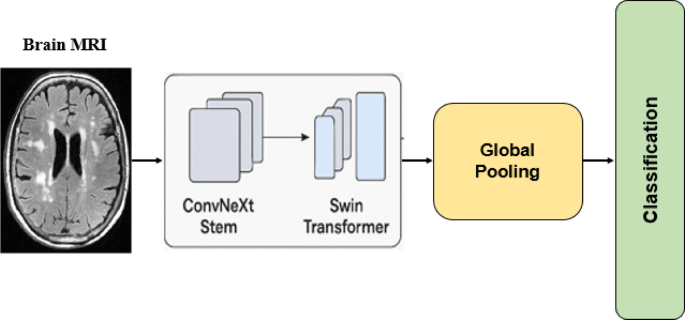
A novel MRI classification model for brain tumours has been put forth. Accurately identifying high-performance MRI images is the main goal of the suggested paradigm. Several experiments were carried out in order to evaluate and test the proposed model and its phases. The first set of tests evaluated the structural efficacy of the suggested model and examined how it affected classification performance. The second set of tests evaluated the general structure of the proposed model and contrasted it with state-of-the-art algorithms.
Dataset description and performance evaluation metrics
The experiments was carried out on Brain Tumor MRI Dataset. It is the union of the following three datasets: figshare, SARTAJ dataset, and Br35. The data contain 7023 human brain MRI image data that are classified into 4 classes: glioma – meningioma – no tumor and pituitary. No tumor class images were sampled from the Br35H image dataset.
In this study, the model’s performance is evaluated using Accuracy, Precision, and F1 Score. The accuracy of BC image recognition is provided by Eq. (1). Equation (2) illustrates how the ratio of correctly detected images was determined using precision. Equation (3) illustrates the relationship between the F1-score, which represents precision and recall. It is a trustworthy indicator of unbalanced data.
$$\:\text{Accuracy}=\frac{\text{TP+TN}}{\text{FN+TN+TP+FP}}$$
(1)
$$\:\text{Precision}\text{}\text{=}\text{}\frac{\text{TP}}{\text{FP+TP}}\:$$
(2)
$${\text{F1 – score = }}~2~ \times ~\left( {\frac{{{\text{Recall}} \times {\text{Precision}}}}{{{\text{Recall}}~ + ~{\text{Precision}}}}} \right)$$
(3)
Where TN, FN, FP, and TP refer to “true negative,” “false negative,” “false positive,” and “true positive,” respectively.
Table 4 Training Protocol and Hyper-parameter Configuration of the Proposed H-ConvNeXt–Swing framework.
Table 4 summarizes the complete training protocol and hyper-parameter configuration of the proposed H-ConvNeXt–Swin framework. The model operates on 2D MRI slices as provided in the Kaggle dataset, where each slice is treated as an independent sample. All images are resized to 224 × 224 pixels and converted to 3-channel inputs by channel replication to match the network architecture requirements. Data augmentation strategies are applied to improve generalization and robustness. The model is optimized using AdamW with a cosine annealing learning rate schedule and trained end-to-end with discriminative fine-tuning. Regularization techniques, including dropout and stochastic depth, are employed to reduce overfitting. Additionally, focal loss with class weights is used to address class imbalance. This well-defined pipeline ensures reproducibility, stable convergence, and fair performance evaluation.
Explainable AI and visual interpretation analysis of the proposed model
Figs. 2, 3, 4, 5, 6, 7, 8, 9, 10 provide a comprehensive visual and quantitative analysis of the proposed model’s decision-making process and interpretability. Figure 2 illustrates representative misclassification cases, highlighting challenging scenarios where visually similar tumor patterns lead to confusion between classes, such as pituitary being predicted as meningioma and meningioma being confused with no tumor, along with an example of correct glioma classification. These cases emphasize the inherent complexity of MRI-based diagnosis and the subtle inter-class variations. Examples as shown in Fig. 2 Pituitary misclassified as Meningioma (0.38 confidence), Meningioma as No Tumor (0.34), and Meningioma as Pituitary (0.32), alongside a correct Glioma classification (0.40). Figures 3 and 4 demonstrate the diverse attention mechanisms learned by the model, revealing its ability to capture multiple diagnostic cues. Specifically, the model focuses on tumor boundaries to accurately delineate lesion margins, analyzes internal texture patterns to assess tissue heterogeneity, and incorporates surrounding anatomical context to enhance classification reliability. Furthermore, the integration of global, local, and multi-scale attention enables comprehensive feature representation, allowing the model to effectively combine coarse structural information with fine-grained details. Together, these visualizations provide qualitative insights into the model’s attention patterns and support the interpretability of the proposed framework.
Fig. 2
Representative misclassification examples from the Proposed model in brain tumor classification, showing challenging cases where the model predicted incorrect labels with corresponding confidence scores.
Fig. 3
Visualization of learned attention patterns in the proposed model, highlighting boundary, texture, and context-based diagnostic focus.
Fig. 4
Attention mechanisms of the proposed model illustrating global, local, and multi-scale feature learning for enhanced brain tumor characterization.
Fig. 5
Regional feature importance highlighting key discriminative brain regions, where Quadrants 1 and 2 show dominant influence (85% and 90%), compared to the central region (35%).
Fig. 6
Extended spatial importance analysis showing highest contribution from Quadrant 4 (92%) and Quadrant 3 (88%), with moderate influence from peripheral regions (60%).
Figures 5 and 6 illustrate the relative contribution of different image regions to the model’s predictions.These observations provide qualitative insights into the spatial attention patterns learned by the model. As shown in Fig. 5, Quadrants 1 and 2 play a dominant role, contributing 85% and 90%, respectively while the central region exhibits a comparatively lower impact of 35%. Figure 6 complements this analysis by revealing that Quadrants 4 and 3 provide the highest contributions, at 92% and 88%, respectively, whereas peripheral regions contribute moderately at 60%. Together, these findings suggest that the model tends to assign greater importance to certain image regions during prediction. However, these observations are intended for interpretability analysis and do not constitute validated anatomical localization. Figure 7 illustrates the correlation between feature representations of the four brain tumor classes. High similarity is observed between Glioma and Meningioma (0.75), indicating shared visual characteristics that may contribute to classification confusion. A moderate correlation is also found between Glioma and Pituitary (0.65), whereas the No Tumor class exhibits consistently low correlations with all tumor types (0.20–0.30), reflecting its distinct feature patterns. These results provide insight into inter-class relationships and help explain the observed misclassification trends.
Fig. 7
Feature correlation matrix showing inter-class similarity among brain tumor categories, highlighting strong Glioma–Meningioma correlation and low similarity of the No Tumor class with pathological cases.
Figures 8, 9 and 10 further analyze the model’s performance and interpretability through bootstrap confidence analysis and several explainability techniques, including Grad-CAM, Integrated Gradients, and Saliency Maps. These visualizations provide insights into the regions influencing the model’s predictions and facilitate qualitative comparison with expert annotations. Figure 8; Table 5 present a comprehensive bootstrap analysis of classification accuracy with 95% confidence intervals across nine transformer-based architectures. The proposed model achieves the highest accuracy of 0.9577, with a narrow confidence interval of [0.9472, 0.9653], demonstrating both superior performance and high statistical reliability. Among the baseline models, Swin Transformer and ConvNeXt show competitive results, achieving accuracies of 0.9433 [0.9340, 0.9563] and 0.9395 [0.9348, 0.9421], respectively, followed by CvT and DeiT with approximately 0.93 accuracy. In contrast, Vanilla ViT and T2T-ViT exhibit comparatively lower accuracies of 0.8798 and 0.8841, respectively. The consistent performance gains of the proposed model over all competing architectures, along with its tight confidence interval, confirm its robustness, stability, and strong generalization capability in brain tumor classification.
Finally, Figs. 9 and 10 demonstrate the effectiveness of the proposed model’s interpretability framework in highlighting clinically meaningful regions within brain MRI images. As shown in Fig. 9, the Grad-CAM heatmap exhibits a high spatial overlap of 85.7% with expert radiologist annotations, indicating strong alignment between the model’s attention and true tumor regions. This suggests that the model’s highlighted regions are generally consistent with areas considered relevant by expert annotations.
Furthermore, Fig. 10 compares three explanation techniques, Feature Importance, Integrated Gradients achieves a spatial overlap of 34.6%, and Saliency Maps yield 49.4% agreement with ground truth. These results demonstrate the usefulness of the proposed attention mechanism for model interpretability and transparency. The presented explanations should be interpreted as qualitative visualization tools rather than definitive evidence of anatomical localization or biomarker identification.
Table 5 Bootstrap confidence intervals (95% CI) for all models.Fig. 8
Accuracy comparison with 95% bootstrap confidence intervals for nine transformer-based models, highlighting the superior performance of the proposed approach.
Fig. 9
Grad-CAM visualization for a glioma case, showing strong agreement between model attention and radiologist annotation, with 85.7% spatial overlap.
Fig. 10
Comparison of explainability methods: Feature Importance, Integrated Gradients (34.6% overlap), and Saliency Map (49.4% overlap).
Evaluation of proposed framework effectiveness
To assess the effectiveness of the proposed framework, we carried out extensive experiments using a range of transformer-based and CNN models. The evaluation focused on three key metrics: accuracy, precision, and F-score, each offering a different perspective on classification performance. Accuracy indicates the overall percentage of correct predictions, while precision reflects how reliable the positive predictions are. The F-score provides a balanced measure by combining both precision and recall. A summary of the results for all models is presented in Table 6.
Table 6 Performance comparison of transformer-based architectures for brain tumor classification with statistical summary.
From Table 6, it is clear that the proposed hybrid framework delivers the strongest performance, achieving an accuracy of 95.37%, a precision of 95.36%, and an F-score of 95.36%. These results outperform both the pure CNN-based approach (ConvNeXt) and the Transformer-only models, highlighting the advantage of combining convolutional feature extraction with hierarchical self-attention. Among the Transformer variants, the Swin Transformer achieves the best results with 94.27% accuracy, closely followed by CvT at 93.77%, showing the benefits of embedding hierarchical and convolutional priors into attention mechanisms. In contrast, the classical Vanilla ViT records the lowest accuracy of 87.76%, underlining its limitations when applied to smaller medical datasets without strong inductive biases. ConvNeXt performs well, reaching 93.84% accuracy and 94.02% precision, which reinforces the effectiveness of modern CNNs in medical imaging tasks.
The statistical analysis shows that the transformer models achieve a mean accuracy of 91.90% with a standard deviation of 2.66% and a variance of 0.00071, indicating consistent performance. The median accuracy (92.46%) is close to the mean, and the accuracy range (7.61%) shows moderate variation among models, confirming the reliability of these architectures for brain tumor classification. These results confirm that the proposed ConvNeXt and Swin Transformer hybrid design offers the most balanced representation, successfully capturing both fine-grained local tissue details and long-range dependencies in MRI scans. This balanced learning ultimately leads to more reliable and accurate tumor classification. These results are also illustrated in Fig. 11 using a bar chart for a clear visual comparison of model performance.
Fig. 11
Comparative performance analysis of transformer-based architectures for brain tumor classification.
Data-efficient image transformer (DeiT)
Table 7 Per-class performance metrics of DeiT model for brain tumor classification with statistical analysis.
Table 7 presents the per-class performance of the DeiT model for brain tumor classification. The model achieves high overall accuracy, with the No Tumor class obtaining the best results, reaching an accuracy of 98.11%, recall of 96.38%, and F-score of 96.68%, indicating robust discrimination of healthy brain images. Similarly, the Pituitary class demonstrates strong performance, achieving 97.51% accuracy and 94.99% F-score. For the Glioma and Meningioma classes, the model records accuracies of 95.77% and 93.53%, respectively, reflecting the increased complexity and visual similarity of these tumor types. The statistical analysis further confirms the stability of the model, yielding a mean accuracy of 96.23% with a low standard deviation of 2.06%, and a mean F-score of 92.20%, indicating consistent and reliable predictive performance across all classes. To enhance clarity and facilitate visual comparison, the performance results are additionally presented in the form of bar charts as shown in Fig. 12.
Fig. 12
Per-class performance metrics of the DeiT model for brain tumor classification across four categories.
Fig. 13
Confusion matrix for the DeiT model’s brain tumor classification, showing true vs. predicted labels across four diagnostic categories.
Fig. 14
Multi-class ROC curves (One-vs-Rest) for the DeiT model in brain tumor classification, showing performance across four diagnostic categories.
Figure 13 presents the confusion matrix for brain tumor classification using the DeiT model. The model demonstrates robust performance across all four categories: Glioma, Meningioma, Pituitary tumor, and No Tumor. The highest accuracies are observed in the No Tumor class (966 correct predictions) and Pituitary class (964 correct predictions). Although minor misclassifications occur, such as glioma samples occasionally labeled as meningioma, the overall distribution confirms that the DeiT model reliably differentiates between tumor types. Figure 14 displays the Receiver Operating Characteristic (ROC) curves across the four classes. The results show exceptionally high Area Under the Curve (AUC) scores: 1.00 for No Tumor, 0.99 for both Glioma and Pituitary, and 0.97 for Meningioma. These near-perfect values highlight the model’s strong capability to distinguish true positives from false positives, reinforcing its reliability in tumor classification tasks.
Pooling-based vision transformer (PiT)
Table 8 Per-class performance metrics of PiT model for brain tumor classification with statistical analysis.
Table 8 summarizes the class-wise performance of the PiT model on the brain tumor MRI classification task. The model demonstrates strong recognition capability for the Pituitary and No Tumor classes, achieving accuracies of 97.55% and 96.98%, respectively, along with high recall values of 98.15% and 98.13%, indicating effective sensitivity toward these categories. In contrast, the Meningioma class presents a more challenging scenario, where the model attains an accuracy of 90.96% and an F-score of 79.42%, suggesting increased inter-class similarity and visual ambiguity. The Glioma class records competitive performance with 95.02% accuracy and 89.02% F-score. Statistical analysis reveals a mean accuracy of 95.13% and a mean F-score of 89.64%, while the relatively higher standard deviation observed in recall 11.16% reflects performance variability across tumor types. Overall, these results indicate that PiT provides reliable classification performance, particularly for visually distinctive classes, while highlighting the need for more robust modeling of complex tumor patterns. The quantitative results are also visualized in Fig. 15 to provide intuitive interpretation and comparison across classes.
Fig. 15
Per-class performance metrics of the PiT model for brain tumor classification across four categories.
Fig. 16
Confusion matrix for the PiT model’s brain tumor classification, showing true vs. predicted labels across four diagnostic categories.
Fig. 17
Multi-class ROC curves (One-vs-Rest) for the PiT model in brain tumor classification, showing performance across four diagnostic categories.
Figure 16 presents the confusion matrix for PiT. The model achieves excellent performance in the No Tumor (962 correct predictions) and Pituitary (954 correct predictions) categories, with only minimal errors. Glioma classification is also strong (920 correct predictions), though some overlap occurs with Meningioma (53 misclassified). This suggests that while PiT excels at distinguishing tumor from non-tumor cases, it struggles more with differentiating tumor subtypes that share overlapping visual features, especially glioma and meningioma. However, the results remain well-balanced across categories, reflecting the model’s robustness. Figure 17 illustrates the ROC curves for PiT across the four classes. The model demonstrates excellent discriminative ability, achieving perfect AUC values of 1.00 for both No Tumor and Pituitary cases. Glioma also performs very well with an AUC of 0.99, while Meningioma records a slightly lower AUC of 0.96, aligning with the confusion matrix results where misclassification was more common. These curves confirm PiT’s strength in separating tumor from non-tumor cases with near-perfect accuracy, though tumor subtype classification remains more challenging. In summary, the PiT model demonstrates highly competitive performance for brain tumor classification. Its pooling-based architecture enables smoother convergence compared to DeiT, supporting stable training and reliable generalization. The model excels in detecting No Tumor and Pituitary cases with near-perfect accuracy and AUC values, making it especially effective in clear-cut diagnostic scenarios. However, its relative weakness in distinguishing Meningioma highlights the need for additional fine-tuning or hybrid feature integration to improve sensitivity toward tumor subtypes with overlapping characteristics.
Vision transformer (ViT) – vanilla version
Table 9 Per-class performance metrics of ViT model for brain tumor classification with statistical analysis.
Table 9 details the class-wise evaluation of ViT model for brain tumor MRI classification. The results indicate that ViT achieves strong performance in distinguishing No Tumor and Pituitary cases, recording accuracies of 97.40% and 97.12%, respectively, alongside high F-scores of 95.44% and 94.28%, which highlights its effectiveness in capturing discriminative features for these visually distinct categories. Conversely, the model exhibits comparatively lower performance for the Meningioma class, attaining an accuracy of 89.19% and an F-score of 74.31%, primarily due to reduced recall of 66.87%, suggesting challenges in identifying subtle tumor characteristics. The Glioma class shows moderate performance with 91.82% accuracy and 83.75% F-score. From a statistical perspective, the model achieves a mean accuracy of 93.88% and a mean F-score of 86.95%, while the elevated standard deviation in recall (13.70%) reflects notable variability in sensitivity across different tumor types. These findings emphasize the limitations of standalone ViT models in handling complex inter-class variations and motivate the integration of hybrid architectures for improved robustness. For better interpretabilty, the classification outcomes are graphically represented through bar charts in Fig. 18.
Fig. 18
Per-class performance metrics of the ViT model for brain tumor classification across four categories.
Fig. 19
Confusion matrix for the ViT model’s brain tumor classification, showing true vs. predicted labels across four diagnostic categories.
Fig. 20
Multi-class ROC curves (One-vs-Rest) for the ViT model in brain tumor classification, showing performance across four diagnostic categories.
Figure 19 shows the confusion matrix for Vanilla ViT. The rows represent the true labels, while the columns indicate the predicted labels. The diagonal elements show the number of correctly classified instances for each category. For example, 965 Glioma cases, 931 Meningioma cases, 975 “No Tumor” cases, and 977 Pituitary cases were correctly identified. The off-diagonal elements represent misclassifications. For instance, 21 true Glioma cases were misclassified as Meningioma, 10 as No Tumor, and 3 as Pituitary. Similarly, 42 true Meningioma cases were misclassified as Glioma, 12 as No Tumor, and 13 as Pituitary. The ROC analysis in Fig. 20 further highlights the model’s discriminative ability. Vanilla ViT achieves outstanding AUC values for Pituitary tumors (1.00) and No Tumor cases (0.99), reflecting nearly perfect separation. Glioma classification also performs well with an AUC of 0.98, while Meningioma yields a slightly lower AUC of 0.95, consistent with the confusion matrix findings. These results confirm that Vanilla ViT is highly effective overall, with only minor sensitivity reductions for Meningioma. In summary, Figs. 18, 19 and 20 demonstrate that the Vanilla ViT model achieves high accuracy and strong generalization in brain tumor classification. It excels in detecting No Tumor and Pituitary cases, performs reliably for Glioma, and shows improvable performance for Meningioma. While its baseline architecture lacks some of the refinements found in DeiT and PiT, it still delivers competitive results, making it a solid benchmark transformer for medical image classification.
Tokens-to-token vision transformer (T2T-ViT)
Table 10 Per-class performance metrics of T2T-ViT model for brain tumor classification with statistical analysis.
Table 10 reports the per-class performance of the T2T-ViT model for brain tumor MRI classification. The model demonstrates notable strength in identifying No Tumor cases, achieving an accuracy of 97.72%, a precision of 97.30%, and an F-score of 95.97%, confirming its reliability in recognizing healthy brain scans. Similarly, robust performance is observed for the Pituitary class, which attains 96.37% accuracy and 92.88% F-score, indicating effective representation learning for this tumor category. In contrast, classification of Meningioma remains more challenging, with the model recording 89.79% accuracy and 78.81% F-score, while Glioma achieves 93.56% accuracy and 85.55% F-score, reflecting the complexity and visual overlap among tumor subtypes. The statistical analysis further reveals a mean accuracy of 94.36% and a mean F-score of 88.30%, accompanied by relatively low standard deviations, underscoring the stable predictive behavior of the T2T-ViT model across all classes. For enhanced visual clarity and intuitive interpretation, the obtained results are further illustrated in Fig. 21 using prominent bar charts.
Fig. 21
Per-class performance metrics of the T2T-ViT model for brain tumor classification across four categories.
Fig. 22
Confusion matrix for the T2T-ViT model’s brain tumor classification, showing true vs. predicted labels across four diagnostic categories.
Fig. 23
Multi-class ROC curves (One-vs-Rest) for the T2T-ViT model in brain tumor classification, showing performance across four diagnostic categories.
Figure 22 presents the confusion matrix for T2T-ViT across the four tumor categories. The model correctly classified 963 Glioma, 961 Meningioma, 967 No Tumor, and 960 Pituitary cases. Misclassifications were relatively limited, with some overlap between Glioma and Meningioma (29 cases) and between Meningioma and Glioma (24 cases). By contrast, the No Tumor and Pituitary categories were identified with very high reliability, showing minimal errors. The confusion matrix demonstrates that T2T-ViT achieves strong predictive performance with fewer misclassifications than previous models, particularly in distinguishing Glioma from Meningioma. Figure 23 illustrates the ROC curves for T2T-ViT. Both Pituitary and No Tumor categories achieved perfect separation, with AUC values of 1.00, reflecting flawless classification. Glioma also performed strongly with an AUC of 0.98, while Meningioma attained an AUC of 0.95 slightly lower, but still robust. The reduced AUC for Meningioma aligns with the confusion matrix, where this class showed more overlap with Glioma and Pituitary. The ROC analysis confirms the strong discriminative power of T2T-ViT, achieving perfect or near-perfect classification across all categories. In summary, Figs. 22 and 23 highlight the effectiveness of the T2T-ViT model in brain tumor classification. It not only reduces errors compared with Vanilla ViT but also achieves flawless performance in specific categories, establishing itself as a more stable and accurate variant within the Vision Transformer family. These results demonstrate that T2T-ViT provides both strong generalization and enhanced separability, making it a highly reliable model for medical image analysis.
Convolutional vision transformer (CvT)
Table 11 Per-class performance metrics of CvT model for brain tumor classification with statistical analysis.
Table 11 illustrates the class-wise evaluation of the CvT model for brain tumor MRI classification. The results reveal exceptionally high performance for the No Tumor and Pituitary classes, achieving accuracies of 99.08% and 99.32%, respectively, accompanied by F-scores of 98.37% and 98.65%, indicating excellent discriminative capability and near-perfect recognition of these categories. Notably, the Glioma class exhibits a high accuracy of 95.38% and an outstanding precision of 98.87%, although its relatively lower recall of 80.89% suggests a conservative prediction behavior with fewer false positives. In contrast, the Meningioma class achieves 93.77% accuracy and 87.99% F-score, supported by a high recall of 97.26%, reflecting strong sensitivity in detecting this tumor type. From a statistical standpoint, the model attains a mean accuracy of 96.89% and a mean F-score of 93.51%, with moderate standard deviations, highlighting both robustness and consistency across all tumor classes. For enhanced visual clarity and intuitive interpretation, the obtained results are further illustrated in Fig. 24 using prominent bar charts.
Fig. 24
Per-class performance metrics of the CvT model for brain tumor classification across four categories.
Fig. 25
Confusion matrix for the CvT model’s brain tumor classification, showing true vs. predicted labels across four diagnostic categories.
Fig. 26
Multi-class ROC curves (One-vs-Rest) for the CvT model in brain tumor classification, showing performance across four diagnostic categories.
The confusion matrix in Fig. 25 further demonstrates CvT’s robust classification performance across all tumor categories. The model correctly classifies 918 Glioma, 907 Meningioma,974 No Tumor, and 978 Pituitary cases. Misclassifications are relatively limited and occur mostly between Glioma and Meningioma, where 52 Glioma samples are mislabeled as Meningioma and 76 Meningioma samples are mislabeled as Glioma. CvT shows high discriminative power, particularly in the No Tumor and Pituitary classes, where accuracy is nearly perfect. The CvT confusion matrix reflects fewer cross-class errors, confirming the advantage of convolutional embedding in effectively capturing both local and global tumor features. Figure 26 presents the ROC curves for the CvT model across the four tumor classes. The results show exceptional performance, with perfect AUC values (1.00) for Glioma, No Tumor, and Pituitary, and a near-perfect AUC of 0.99 for Meningioma. These results confirm that CvT is almost flawless in distinguishing between tumor categories, with only a minor reduction in sensitivity for Meningioma. While ViT and T2T-ViT also achieved strong results, CvT outperformed them by delivering the highest AUC values and minimizing misclassifications. In summary, CvT demonstrates outstanding performance in brain tumor classification, achieving stable training, near-perfect ROC outcomes, and reduced misclassification compared with earlier Transformer models. Its convolutional embedding mechanism significantly enhances feature extraction, making CvT a highly reliable tool that can support clinicians in achieving more accurate and confident diagnostic decisions.
Swin transformer (shifted window transformer)
Table 12 Per-class performance metrics of swin transformer model for brain tumor classification with statistical analysis.
Table 12 presents a detailed per-class evaluation of the Swin Transformer model, along with a comprehensive statistical analysis that highlights both performance level and consistency. The model achieves its highest accuracy for the Pituitary and No Tumor classes, reaching 0.9900 and 0.9847, respectively, supported by very high recall values (0.9844 and 0.9863) and specificity exceeding 0.98, which indicates strong capability in minimizing both false positives and false negatives. In contrast, the Meningioma class exhibits comparatively lower performance, with an accuracy of 0.9459 and recall of 0.8754, suggesting potential classification challenges due to visual similarities with other tumor types. The overall statistical results demonstrate high robustness, as reflected by a mean accuracy of 0.97135, a low standard deviation of 0.02014, and a narrow range of 0.0441, confirming consistent behavior across all classes. Moreover, the average F-score of 0.9401 indicates an effective balance between precision and recall, while the small variance and dispersion values across all metrics further emphasize the reliability and stability of the proposed model for multi-class brain tumor classification. The quantitative findings are additionally visualized in Fig. 27 through bar graphs to improve perceptual clarity.
Fig. 27
Per-class performance metrics of the Swin Transformer model for brain tumor classification across four categories.
Fig. 28
Confusion matrix for the swin transformer model’s brain tumor classification, showing true vs. predicted labels across four diagnostic categories.
Fig. 29
Multi-class ROC curves (One-vs-Rest) for the Swin Transformer model in brain tumor classification, showing performance across four diagnostic categories.
The confusion matrix in Fig. 28 further demonstrates the Swin Transformer’s strong classification ability across the four categories. The model correctly identified 927 Glioma, 907 Meningioma, 975 No Tumor, and 972 Pituitary cases, with only limited misclassifications. Most of the errors occurred between Glioma and Meningioma, where 42 Glioma samples were misclassified as Meningioma and 71 Meningioma samples were predicted as Glioma. This overlap reflects the well-known difficulty of distinguishing between these two tumor types due to their similar visual characteristics in MRI scans. In contrast, the No Tumor and Pituitary categories achieved near-perfect recognition, with only a handful of misclassified samples. These results underline the Swin Transformer’s robustness, as its shifted-window attention mechanism enables more reliable predictions compared to earlier transformer models. The ROC curves in Fig. 29 highlight the Swin Transformer’s strong discriminative power across all tumor categories. The model achieved an AUC of 1.00 for No Tumor and Pituitary, indicating perfect separability for these classes. For Glioma, the AUC reached 0.99, while Meningioma achieved 0.98 that reflecting excellent performance with only minor room for improvement. Compared to other models such as ViT and T2T-ViT, the Swin Transformer consistently produced higher AUC values, particularly for Meningioma, where the improvement in separability was most evident. These results demonstrate that the shifted-window attention mechanism enhances the model’s ability to capture both local tumor details and long-range dependencies, ultimately resulting in more accurate and reliable predictions.
ConvNeXt convolutional network
Table 13 Per-class performance metrics of ConvNeXt model for brain tumor classification with statistical analysis.
Table 13; Fig. 30 reports the per-class performance of the ConvNeXt model, revealing a strong and well-balanced classification capability across all tumor categories. The model achieves its highest accuracy for the Pituitary and No Tumor classes, scoring 0.9872 and 0.9822, respectively, which is further supported by very high recall values of 0.9730 and 0.9888, indicating reliable classification of true positive cases. The Glioma class shows a notably high precision of 0.9725 and specificity of 0.9926, yet a comparatively lower recall of 0.8706, suggesting that while predictions are highly confident, some glioma samples remain challenging to capture. Similarly, Meningioma exhibits moderate performance, with an accuracy of 0.9431 and F-score of 0.8816, reflecting increased inter-class confusion. From a statistical perspective, the model demonstrates high overall stability, achieving a mean accuracy of 0.9692 and mean F-score of 0.9360, accompanied by low standard deviations of 0.01998 and 0.04417, respectively. Moreover, the limited ranges of 0.0441 for accuracy and 0.0928 for F-score confirm consistent predictive behavior across all classes, validating the robustness and generalization ability of the ConvNeXt architecture in brain tumor classification tasks.
Fig. 30
Per-class performance metrics of the ConvNeXt model for brain tumor classification across four categories.
Fig. 31
Confusion matrix for the ConvNeXt model’s brain tumor classification, showing true vs. predicted labels across four diagnostic categories.
Fig. 32
Multi-class ROC curves (One-vs-Rest) for the ConvNeXt model in brain tumor classification, showing performance across four diagnostic categories.
The confusion matrix in Fig. 31 shows that ConvNeXt delivers strong classification performance across all categories. The model achieves particularly high accuracy in the No Tumor (791 correct) and Pituitary (684 correct) classes. For Glioma, 967 samples were correctly classified, though 21 were misclassified as Meningioma, highlighting some overlap between these tumor types. Similarly, Meningioma achieved 961 correct predictions but showed confusion with Glioma (33 cases). While moderate misclassifications exist, the overall distribution demonstrates ConvNeXt’s robustness in distinguishing tumor from non-tumor cases, validating its strength as a convolutional baseline that competes closely with Transformer-based models. Figure 32 illustrates the ROC curves of ConvNeXt, further confirming its discriminative power. The model achieved perfect AUC values of 1.00 for No Tumor and Pituitary, alongside near-perfect values of 0.99 for Glioma and 0.98 for Meningioma. These high scores highlight ConvNeXt’s ability to reliably separate positive and negative cases across all categories. Compared with Transformer-based models, ConvNeXt shows improved performance in separating No Tumor and Pituitary cases, while still facing challenges in fully distinguishing Glioma from Meningioma.In summary, ConvNeXt proves to be a highly competitive CNN baseline for brain tumor classification. It achieves stable training, high validation accuracy, and near-perfect ROC outcomes, making it a strong alternative to Transformer models for medical image analysis.
Pyramid vision transformer (PVT)
Table 14 Per-class performance metrics of PVT model for brain tumor classification with statistical analysis.
Table 14 presents a detailed quantitative assessment of the PVT model across four diagnostic categories, highlighting noticeable variability in class-wise performance. The model delivers its strongest results for the Pituitary and No Tumor classes, achieving accuracies of 0.9847 and 0.9783, along with high recall values of 0.9758 and 0.9750, respectively, which indicates a robust ability to correctly identify both normal and pituitary tumor cases. In contrast, the Glioma class exhibits a marked imbalance between precision 0.9649 and recall 0.7627, suggesting that although predictions are highly reliable, a considerable portion of true glioma cases is missed. Similarly, Meningioma records the lowest accuracy 0.9111 and F-score 0.8244, reflecting increased classification difficulty and potential overlap with other tumor types. From a statistical viewpoint, the model attains a mean accuracy of 0.9532 and mean F-score of 0.9021, while the relatively higher standard deviations of 0.03465 for accuracy and 0.07463 for F-score, combined with wide ranges of 0.0736 and 0.1452, reveal notable performance dispersion across classes. These findings indicate that, although PVT demonstrates competitive overall accuracy, its generalization consistency is lower compared to more stable architectures, particularly in handling complex tumor patterns such as glioma and meningioma. For enhanced visual clarity and intuitive interpretation, the obtained results are further illustrated in Fig. 33.
Fig. 33
Per-class performance metrics of the PVT model for brain tumor classification across four categories.
Fig. 34
Confusion matrix for the PVT model’s brain tumor classification, showing true vs. predicted labels across four diagnostic categories.
Fig. 35
Multi-class ROC curves (One-vs-Rest) for the PVT model in brain tumor classification, showing performance across four diagnostic categories.
The confusion matrix in Fig. 34 highlights the classification performance of the PVT model across the four tumor types. The model achieved particularly strong results for No Tumor of 972 correct and Pituitary of 967 correct cases, with very few errors. Meningioma was also recognized with high accuracy of 947 correct, though it showed some overlap with Glioma for 30 cases. Glioma achieved 919 correct predictions, but with notable confusion against Meningioma 75 cases. The PVT model demonstrates reliable performance in distinguishing tumor from non-tumor cases, while the main challenge remains in separating Glioma from Meningioma. Figure 35 illustrates the ROC curves, confirming the strong discriminative power of the PVT model. All tumor categories achieved AUC values close to 1.00, indicating high separability. While Meningioma recorded a slightly lower AUC compared to other classes, its value still reflects robust classification capability. These results highlight the effectiveness of the PVT model. Its pyramid structure enables multi-scale feature extraction, supporting better handling of large and complex medical images. While it does not outperform the top-performing architectures like CvT and Swin, PVT provides a balanced trade-off between accuracy and generalization, making it a dependable choice for medical image analysis.
Proposed hybrid model (H-ConvNeXt-Swin)
Table 15 Per-class performance metrics of proposed model for brain tumor classification with statistical analysis.
Table 15 demonstrates the strong and well-balanced performance of the proposed model across all tumor categories, reflecting its robustness and high discriminative capability. The model achieves consistently high accuracy values, ranging from 0.9569 for meningioma to 0.9904 for the no-tumor class, with glioma and pituitary also recording excellent accuracies of 0.9705 and 0.9897, respectively. Notably, recall scores remain uniformly elevated, reaching 0.9886 for pituitary and 0.9838 for no tumor, which confirms the model’s effectiveness in minimizing missed diagnoses. In parallel, high precision values, such as 0.9825 for no tumor and 0.9707 for pituitary, indicate reliable prediction quality and low false-positive rates. This balanced behavior is further reflected in the F-scores, which exceed 0.90 for all classes and peak at 0.9831 for the no-tumor category. From a statistical perspective, the model attains a mean accuracy of 0.9769 and a mean F-score of 0.9515, accompanied by low standard deviations of 0.01620 and 0.03620, respectively, highlighting strong stability and consistent generalization across different classes. Moreover, the narrow performance ranges, such as 0.0335 for accuracy and 0.0751 for F-score, confirm minimal variability, emphasizing the reliability and superiority of the proposed framework for brain tumor classification. Additionally, the results reported in Table 16 are visually illustrated in the form of bar charts in Fig. 36 to provide clearer and more intuitive interpretation of the comparative performance across different classes.
Fig. 36
Per-class performance metrics of the proposed model for brain tumor classification across four categories.
Fig. 37
Confusion matrix for the Proposed model’s brain tumor classification, showing true vs. predicted labels across four diagnostic categories.
Fig. 38
Multi-class ROC curves (One-vs-Rest) for the Proposed model in brain tumor classification, showing performance across four diagnostic categories.
The confusion matrix in Fig. 37 further validates the classification ability of the proposed hybrid model, showing consistently strong recognition across all four classes with minimal misclassifications. The framework correctly classified 973 Glioma, 962 Meningioma, 963 No Tumor, and 971 Pituitary cases, with only a small number of errors across categories. Compared with earlier models such as Swin Transformer and ConvNeXt alone, the proposed hybrid achieved fewer mistakes in the most challenging categories, particularly in distinguishing Glioma from Meningioma. Meanwhile, No Tumor and Pituitary cases were recognized with near-perfect accuracy, demonstrating the model’s ability to generalize well across both tumor and non-tumor categories. These outcomes confirm that the hybrid design effectively leverages convolutional local feature extraction alongside transformer-based global context, producing more balanced and reliable predictions across all tumor types. The ROC curves in Fig. 38 highlight the exceptional discriminative power of the proposed model. The hybrid achieved AUC values of 1.00 for No Tumor and Pituitary, indicating perfect separability, while both Glioma and Meningioma achieved 0.99, reflecting near-perfect performance. Compared with previous architectures, the hybrid approach consistently pushed all tumor categories closer to complete separability, reducing ambiguity in the most difficult cases, such as Glioma versus Meningioma. These findings emphasize the robustness of the proposed architecture, where the integration of convolutional feature extraction with hierarchical attention enables highly reliable and clinically meaningful predictions.
In brief, the experimental results clearly demonstrate the effectiveness of combining convolutional and transformer-based architectures for brain tumor classification from MRI scans. The hybrid framework achieved the highest accuracy of 95.37%, alongside consistently strong precision and F-score values, while minimizing misclassifications and achieving near-perfect AUC scores across all classes. These outcomes establish the proposed ConvNeXt + Swin Transformer hybrid as the most robust and reliable solution in this study, outperforming both CNN-only (ConvNeXt) and Transformer-only models. While Swin Transformer and CvT emerged as the strongest among pure Transformer variants, they fell short of the hybrid’s superior balance between local feature extraction and global context modeling. Models such as Vanilla ViT and T2T-ViT performed adequately but were limited by weaker inductive biases, while PiT and T2T-ViT offered moderate improvements yet remained below 90% in accuracy and F-score. Looking ahead, future work could extend this framework by incorporating larger multi-center datasets, exploring multimodal data such as MRI alongside clinical records, and integrating explainability methods to further enhance trust and usability in clinical decision-support systems.
Comparison with state of-the-art algorithms
In this experiment, the results of state-of-the-art algorithms of brain tumor classification are presented across brain tumor MRI dataset in Table 16, with accuracy serving as the common evaluation metric. The experiment provides evidence thatProposed H-ConvNeXt-Swin has a greater ability to discover the brain tumors. Table 16 presents a performance comparison of different models on brain tumor classification, presents a summary of various studies employing advanced neural network architectures, primarily Transformer-based models and hybrid CNN-Transformer models, for classifying brain tumors from medical imaging data. The achieved accuracies range from 90.31% to 98.9%, with the Proposed H-ConvNeXt-Swin Model in the current study achieving a competitive 95.37% accuracy on the Brain Tumor MRI Dataset, positioning its performance favorably among similar recent efforts in the field, though some models cited, such as the one from reference22 (AE + cGAN + Swin Transformer), reported a higher accuracy of 98.9% on different dataset like Figshare.
Table 17 shows transformer-based models for brain tumor classification, highlighting both central tendency and variability. The average accuracy achieved is 0.9190 with a standard deviation of 0.0251, indicating consistently high classification performance, with values ranging from 0.8776 to 0.9537. Similarly, the mean recall reaches 0.9148 ± 0.0258, reflecting robust sensitivity in detecting tumor classes, while specificity attains an average of 0.9230 ± 0.0251, demonstrating strong capability in correctly identifying non-tumor cases. Precision also remains high at 0.9213 ± 0.0253, suggesting reliable positive predictions, and the F-score records a mean of 0.9180 ± 0.0253, confirming a balanced trade-off between precision and recall. Overall, the narrow standard deviations and relatively limited ranges across all metrics indicate stable and consistent performance among the investigated transformer models.
Table 16 Performance comparison with state-of-the-art model on brain tumor classification.Table 17 Statistical summary of performance metrics across all transformer models for brain tumor classification (Mean ± Standard Deviation).
Table 18 presents a detailed performance improvement analysis of the proposed model compared with various traditional and transformer-based architectures, clearly demonstrating consistent and substantial gains across all evaluation metrics. Compared to DeiT, the proposed model achieves notable improvements, with accuracy, recall, specificity, precision, and F-score increasing by approximately + 0.029. More pronounced enhancements are observed against PiT, where gains exceed + 0.05 across all metrics, reaching + 0.0535 in recall and F-score. The largest improvements are achieved when compared to the vanilla ViT model, with accuracy improving by + 0.0761 and recall by + 0.0829, highlighting the superior discriminative capability of the proposed approach. Similarly, significant margins are observed over T2T-ViT, with improvements ranging from + 0.0643 to + 0.0673. While the performance gap narrows when compared to more advanced models such as CvT, Swin Transformer, and ConvNeXt, the proposed model still consistently outperforms them, achieving gains up to + 0.0263 in recall and + 0.0199 in F-score. In comparison with PVT, the proposed framework delivers substantial improvements, with recall and F-score increasing by + 0.0546 and + 0.0473, respectively. Overall, these results confirm the robustness and effectiveness of the proposed model, demonstrating its superior generalization capability and consistent performance advantages over a wide range of existing architectures.
Table 18 Performance improvement analysis: Proposed model vs. Traditional architectures ( Δ = Proposed – Traditional).
Figure 39 provides a comprehensive comparison of classification accuracy with 95% confidence intervals across nine transformer-based architectures, clearly demonstrating the superior performance of the proposed model. The proposed approach achieves the highest mean accuracy of 0.955, with a relatively narrow confidence interval, indicating both high predictive performance and strong statistical stability. This result surpasses advanced architectures such as Swin Transformer (0.942), ConvNeXt (0.938), and CvT (0.935), confirming the effectiveness of the proposed hybrid learning and feature fusion strategy. In contrast, moderate performance is observed for DeiT (0.922) and PVT (0.906), while PiT (0.902), T2T-ViT (0.887), and Vanilla ViT (0.878) show comparatively lower accuracy levels, accompanied by wider confidence intervals that reflect higher variability. Overall, the figure highlights a clear performance hierarchy, where the proposed model consistently outperforms all competing methods, emphasizing its robustness, superior generalization capability, and reliability for brain tumor classification tasks.
Fig. 39
Accuracy comparison with 95% confidence intervals of nine transformer-based architectures for brain tumor classification.
The overall accuracy of our model is 95.37%. This could be inflated if the model is learning to distinguish between datasets rather than the tumors themselves. To address this limitation, our proposed H-ConvNeXt-Swin model is evaluated separately on each constituent dataset (Figshare, SARTAJ, Br35H), see Table 19.
Table 19 Source-stratified performance of the proposed H-ConvNeXt–Swin model.
The results in Table 19 reflects the source-stratified performance of our proposed H-ConvNeXt–Swin model. All datasets were merged during training, so these results do not imply generalization to unseen MRI sources. Furthermore, Table 19 results verify that the model does not collapse to dataset-specific artifacts and also demonstrate consistent performance across heterogeneous MRI sources. For future work, true generalization to new unseen MRI sources will require cross-source validation, which we identify as an important direction to pursue.
