


GeoMx digital spatial profiling data acquisition
Ovarian Cancer (OC) patient tissue biopsies45 were analyzed using the GeoMx Digital Spatial Profiling platform (Nanostring)24. Ten tissue microarray (TMA) slides, with 4 μm thick cuts of 1 mm diameter formalin-fixed paraffin-embedded tissue cores (3 cores per tumor), were stained with SYTO 13 (nuclear stain) and three fluorescence- labeled antibodies against PanCK (tumor), CD45 (immune cells) and CD8 (cytotoxic T-cells), and panels of photocleavable oligonucleotide-tagged antibodies, as described38. ROIs were selected using the IF images, probes were collected by exposing ROIs to UV light, followed by quantification using nCounter (Nanostring). The protein panel consisted of 78 antibodies specific for immune and tumor markers (Fig. S15), including 6 control markers not included in our predictions. Based on the images of tumor cores from 254 patients, 636 ROIs were selected from representative tumor, stroma or mixed regions. Normalization of ROI protein counts was performed in the GeoMx analysis suite through linear scaling of protein counts based on the geometric mean of housekeeping protein Histone H3. OME-TIFFs were exported from the GeoMx analysis suite and cell segmentation was performed in QuPath with stardist (dsb2018_heavy_augment.pb)46,47.
t-CyCIF data acquisition
The publicly available CRC Atlas 202227,28 (obtained from the author`s github https://github.com/labsyspharm/CRC_atlas_2022) consists of data and images from 17 colorectal cancer (CRC) patients. The samples have been stained using cyclic immunofluorescence (t-CyCIF), generating single-cell resolution stainings of multiple (n = 35) protein markers. DNA staining (Hoechst) was included in each staining cycle; however, we only used the DNA channel from cycle 1. We did not include information from the isotype (negative) control markers. We used data from patients 2–17, consisting of 16 25-plex images, with corresponding spatial data, containing coordinates and marker abundance for each cell. Pseudo-bulk count data were constructed by adding expression based on marker abundance of all cells in a given area to resemble GeoMx data and train model predictions. Note that these visually obtained counts were high (high thousands per protein per cell) compared to GeoMx data (hundreds of protein counts for hundreds of cells together), as they were based on relative fluorescence units, which range between 0 and 65536.
CosMx NSCLC data acquistion
The publicly available CosMx NSCLC data23 (available from Nanostring’s website) consist of CosMx data from eight tissue samples collected from five patients. Tissue had been stained for membrane, PanCK, CD45, CD3 and DAPI, and count data were from a 960-plex CosMx RNA panel. We preprocessed downloaded data into a format compatible with our code, as documented on our github. Dropout of gene counts is a known issue for some spatial omics methods such as CosMx11. We tentatively imputed missing transcripts to investigate how well Image2Count trained on non-imputed data reflects imputed cell counts, using a DCA36 with the following parameters: ae_type was set to zinb_condisp, lr to 0.0005, batch_size to 256 and hidden_size to (256, 128, 64, 128, 256). DCA is an established method for imputing missing counts for single-cell RNA-seq data.
Preprocessing
For the t-CyCIF dataset, cell positions and per-cell mean staining intensities had been made available via the tool MCMICRO48 for all images27. Bottom and top 1% of summed cell expression were filtered to remove outliers. Each cell was then cut out in 50 × 50 (34 × 34 pixels), 20 × 20 (14 × 14 pixels) and 8 × 8 (6 × 6 pixels) μm windows, for different model runs, respectively, for the t-CyCIF dataset. For the GeoMx dataset, cells were cut out in 50 × 50 (124 × 124 pixels), 30 × 30 (74 × 74 pixels), 20 × 20 (50 × 50 pixels), 12 × 12 (30 × 30 pixels) and 8 × 8 (20 × 20 pixels) μm windows, respectively. We do not report on 50 × 50 and 30 × 30 μ m windows as the visual feature encoder overfitted given the GeoMx dataset size (Figure S16). For the CosMx dataset, cells were cut out in 18 × 18 (100 × 100 pixel) μm window. For all training data, channel-specific mean and standard deviation were calculated for normalization purposes. For CosMx 4 (total 732), for t-CyCIF 49 (686 total) equally distributed subgraphs, with an 11-hop neighborhood starting from the central cell (containing on average 384 and 260 cells, respectively), per WSI/patient/fov (field of view) were created for model training. When investigating accuracy for differently sized regions on the test data, 36 subgraphs per fov for CosMx were created (total 1800), 49 per WSI for CRC (total 2700). Region size was varied to 1, 2, 3, 5, 8 or 11 hop subgraphs.
Visual feature extraction
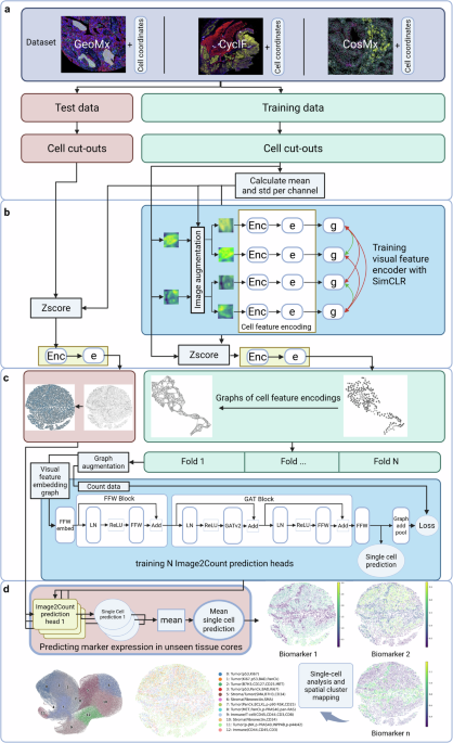
Visual features were extracted via pre-training a ResNet model with the contrastive loss from SimCLR26,49, following similar approaches that extract visual features from multiplex IF images7. ResNet was chosen as an encoder as cell cut-outs consist of low pixel window sizes (from 100 × 100 to 6 × 6 pixels). Datasets with cell cut-outs below 50 × 50 pixels utilized ResNet18, while datasets with cell cut-outs above 50 × 50 pixels and a sufficient number of cells to train on used ResNet50 as an encoder.
The architecture of the ResNet model had to be modified to allow for training with a contrastive loss to work on small images and to handle image data with more or less channels than three. We therefore modified the first Conv2d layer of a ResNet model obtained via PyTorch to input the number of channels we provided (four if not otherwise specified) and changed the kernel size to (3, 3) and stride to 1, as motivated by ref. 26 when working on smaller images. We also followed the recommendation to remove the first max-pooling operation. We did not use these changes when training on images with 74 × 74 pixels or larger. The projection head g(.) was a nonlinear MLP with one hidden layer. However, unlike in the SimCLR paper g did not work on the avgpooling layer output, but followed the implementation of NaroNet and operated on a nonlinear embedding e(.), which does follow the avgpooling layer. This allows for visual features to exist in a smaller feature space e, needed for downstream training and tasks, while performing the contrastive loss on outputs of g, which is conjectured to lose relevant information as g is trained to be more invariant to data transformations26.
Stochastic Gradient Descent was utilized as the optimizer with a weight decay of 1e − 6 (5e − 6 for the GeoMx dataset when training on images of size 50 × 50 μm or larger to combat overfitting), momentum set to 0.9, as well as Nvidia’s apex PyTorch implementation of LARC, following SimCLR26,50,51. Learning rate scheduling was performed with PyTorch’s OneCycleLR52. OneCycleLR scales the learning rate to the given maximum learning rate in a specified fraction of total training epochs, and then decreases it. Updates to the learning rate are performed for every minibatch.
Image augmentation consisted of random cropping and resizing into the original shape, horizontal and vertical flipping, introduction of random artifacts, random background, Gaussian blurring, Gaussian noise and z-score normalization.
During training of the visual feature extraction module, images of cells that were underrepresented in the data were over-sampled to improve features extracted from low-abundance cell types. This was done by first extracting centroid pixels of every image and then performing K-Means elbow on a random subset of 10,000 pixels 5 times to obtain the optimal number of clusters. The optimal number was then used to run K-Means on all image pixel centroids, sampling from every cluster equally during training.
Visual representations of cells for downstream tasks were obtained from e(.) after pre-training the visual feature extraction module once, for all cells in a given training dataset, without further fine-tuning.
Graph learning
Learned cell representations were transformed into a cell graph with squidpy53 by calculating the Euclidean distance to each cell’s 6 nearest neighbors. AdamW54 with a weight decay was utilized to optimize model parameters in this part of the model. Visual representations obtained from the previous step were embedded via a 2-layer MLP, as shown in Fig. 1c in the embedding block. i FFW blocks, built of pre-LayerNorm and ReLU, followed by a two-layer Feed-Forward Network (FFW) and residual connection, further extracted relevant features from the image embeddings. What follows is n GAT55,56 blocks when utilizing GAT Image2Count instead of FFW Image2Count models (see GATv2 block in 1c), consisting of pre-normalization and activation, shown to be beneficial for deep networks57,58, graph attention convolution v2 (utilizing torch geometric) with nheads attention heads, which get concatenated, and afterwards transformed into the original embedding dimension via a linear layer, followed by a residual connection and a FFW Block. Li et al. showed that deep graph convolutional networks benefit, similarly to convolutional neural networks (CNNs), from residual connections59. We therefore incorporated this concept to facilitate the construction of deep models. The resulting GAT blocks are highly similar to modern transformer blocks.
The last part of Image2Count prediction heads consisted of projecting the learned cell representation via a 2-layer MLP onto expression counts, then calculating the exponential of expression counts and clipping values below 1e-5 and above 1e+6 (similar to the mean activation used by Eraslan et al.36). Downstream analysis used this layer as output to obtain single-cell-level expression predictions. While training, all cell expressions of a graph were summed together via a global add pool, which was used to calculate the L1 loss between predicted expressions and the observed bulk counts of the region/graph after calculating their log + 1 values to achieve more stable learning. We also used 1 − CosineSimilarity(x, y) as an additional loss term, as can be seen in Equation 1. Values used for γ1 and γ2 in Equation 1 were always 1.
$$\begin{array}{rcl}{L}_{i}&=&{\gamma }_{1}* L1(\log ({x}_{i}+1),\log ({y}_{1}+1))\\ &&+{\gamma }_{2}* (1-\,{\text{sim}}\,({x}_{i},{y}_{i}))\end{array}$$
(1)
Graphs were constructed via KNN, with each cell having edges to its six nearest neighbors. Edge attributes consisted of the distance between cells and node attributes were the visual feature representations. While training, we made use of multiple graph augmentations: Positional jittering, where cell positions are randomly jittered locally in pixel space and recomputing edges and distances without changing the macro topology; as well as randomly dropping edges and nodes from the graph. Data utilized the same training and test splits used for the visual feature extraction, with training data being further split over patients/slides for cross-validation. Training was stopped when no improvement in loss was observed on validation folds. We compared GAT Image2Count to FFW Image2Count and a linear prediction model. Model parameters were chosen based on coarse manual testing of model performance on training data.
Linear prediction
Linear prediction of gene expression was done through a simple one-layer linear network fR×num_genes. Batch size of 64, learning rate of 0.005, weight decay of 5e − 4, AdamW as optimizer, node dropout of 0.05, early stopping of 25, and tenfold cross-validation were used as parameters for the t-CyCIF dataset. For the GeoMx dataset, the learning rate was adjusted to 0.01; for the CosMx dataset, sixfold cross-validation was used.
CosMx NSCLC Image2Count model
Visual representation learning was performed using all image channels. Cell cut-outs were clustered with K-Means (k = 30) to oversample low-abundance cell types. As base encoder a ResNet50 model was chosen because of the cell cut-out size (18 × 18 μ with 100 × 100 pixels), with batch size of 512, max learning rate of 0.1, 30 warm-up epochs, 300 total epochs, embedding size of 512, loss dimension of 128, data augmentation with default parameters and an additional brightness and contrast augmentation in 80% by randomly adjusting brightness and contrast between 0.5 and 2 for all channels. Lung 6 and Lung 13 were used for test data.
GAT Image2Count prediction head was constructed as follows: 3 linear blocks, 3 GAT blocks, GATv2 node size of 64, 8 attention heads and positional cell jittering of 40. The FFW Image2Count prediction head consisted of 17 linear blocks. Both used batch size of 64, learning rate of 0.0001, an embed node size of 128, weight decay of 5e − 3, early stopping of 25, sixfold cross-validation over slides and an embedding dropout of 0.5. Consensus predictions of the test data were obtained by calculating the mean test prediction over all 6 Image2Count prediction heads.
t-CyCIF CRC Image2Count model
To resemble the GeoMx data, visual representation learning on the t-CyCIF data was done using image channels 0 (Hoechst1), 10 (Keratin), 14 (CD45), and 19 (CD8a). Visual representation learning was also performed on only channel 0 (Hoechst1) and 10 (Keratin) to investigate the benefits of cell type-specific staining for the downstream task. In order to oversample low-abundance clusters during training for a more equal cell class distribution, centroid pixels of each cell cut-out were used for K-Means, with k = 30 for 4-channel and k = 10 for the 2-channel model determined as a good fit number of clusters via the elbow method. ResNet18 was chosen as the encoder as the cell cut-out pixel size was less then 50 × 50, with a batch size of 4096, a max learning rate of 0.1, 10 warm-up epochs and running for 100 epochs. Embedding size of e() was set to 32, while the loss operating on outputs of g() had 16 dimensions. Data augmentation was done with our default parameters. We split the 8.6 million cells into 80% for training and 20% for testing by using WSI 3, 5, and 13 for testing and the rest for training, reaching a test loss accuracy after training of 71.16%, while having a performance of 95.06% on the training set with 50 μm cut-outs. We used the following parameters to construct Image2Count prediction heads: GAT Image2Count was done with 24 linear blocks, 6 GAT blocks, GATv2 node size of 32, 8 attention heads, edge dropout of 0.3, and positional cell jittering of 40. FFW Image2Count consisted of 35 linear blocks. Both Image2Count models used a batch size of 64, a learning rate of 0.0001, an embedded node size of 128, weight decay of 5e − 4, early stopping of 25, tenfold cross-validation over WSI, and embedding dropout of 0.1. The previous train/test split was utilized, performing tenfold cross-validation on the training data (split over patients) and comparing predictions on the test data. We compared our GAT Image2Count model to a FFW Image2Count and a linear prediction head for the frozen visual feature backbone (see section Graph Learning), when training the visual representation backbone with two channels (DNA and Keratin) and four channels (DNA, Keratin, CD45, CD8a), as well as cell cut-out sizes of 8 × 8 and 20 × 20 μm windows instead of 50 × 50 μm. Consensus or merged model predictions of the test data were obtained by taking the mean test prediction of all 10 cross-validation Image2Count prediction heads.
GeoMx OC Image2Count model
A ResNet18 was chosen as an encoder, as cell cut-out size in pixels was below 50 × 50, with a batch size of 1024, max learning rate of 0.1, 95 warm-up epochs and training for 950 epochs. As the GeoMx dataset was smaller than the t-CyCIF dataset, we had to reduce the batch size and increase the number of epochs to achieve similar performance. The embedding dimension of layer e() was set to 32, and the output dimension of g(), upon which the contrastive loss was calculated, was set to 16. Data augmentation was performed using default parameters. The centroid pixel of each cell cut-out was used for K-Means, with k = 20 determined as a good fit number of clusters via the elbow method, to oversample low-abundance clusters during training for a more equal cell class distribution. The ten tumor TMAs were split into a train and test set: seven for training (486 ROIs), three for testing (150 ROIs). The contrastive loss accuracy for the test data was 0.67 after training, and on the training data, 0.88.
Larger areas on slide 1C54, part of the test set, for which no count data was available over the whole area, were segmented via QuPath and Stardist to create single-cell expression predictions from the trained model for inference.
We used the following parameters to construct Image2Count prediction heads: GAT Image2Count used 3 linear blocks, 3 GAT blocks, GATv2 node size of 8, 2 attention heads, edge dropout of 0.3, positional cell jittering of 40. FFW Image2Count consisted of 7 linear blocks. Both Image2Count prediction head models used a batch size of 64, a learning rate of 0.0005, an embedded node size of 32, weight decay of 1e − 2, early stopping of 50, tenfold cross-validation over patients on the training data and embedding dropout of 0.5. Merged model predictions of the test data were obtained by taking the mean test prediction of all cross-validation Image2Count prediction heads. Coarse manual tests confirmed parameters to be a good fit.
Single-cell analysis
After training the FFW/GAT Image2Count prediction head models and linear prediction head for the frozen ResNet, we generated single-cell expression predictions of the test data and performed single-cell analysis. Consensus or merged model predictions of the test data were obtained by taking the mean prediction of all cross-validation models trained on the training data. Single-cell analysis was performed with scanpy37. Count normalization was performed through median count depth normalization followed by a log1p transformation and scaling to unit variance with a mean of zero. Principal Component Analysis (PCA) was then performed using markers whose prediction over all test ROIs had Spearman p-values below 0.05, retaining a maximum of min(number_of_genes, 100) components (for the CRC dataset, we also excluded Hoechst, NaKapTase, CDX2 and Ki67_570). Subsequently, the 10 nearest neighbors were determined based on all principal components. Using the nearest neighbors graph, a Uniform Manifold Approximation and Projection (UMAP) was computed to embed the graph into a two-dimensional space for visualization. Cells were assigned to clusters using Leiden clustering, with a resolution of 0.5 for GeoMx and 0.25 for CRC. Proteins associated with clusters were identified using the Wilcoxon rank-sum test.
To visualize predicted expression of cells and their location in the tissue, we plotted the per-cell count normalized and log1p transformed predicted and normalized original cell signals on top of the corresponding cells in an image or image section with squidpy53, generating a clearer visualization of the predicted and actual spatial distribution of protein expressions.
Comparison metrics
Metrics were calculated on the test data. For CosMx and t-CyCIF datasets, ground truth data was available; therefore, metrics were calculated on the single-cell level and at different neighborhood sizes as described in Preprocessing. Pearson correlation is a linear correlation. Spearman correlation is rank-based, indicating capability to rank differences correctly. MI measures dependency between two variables, with higher values indicating higher dependency. MSE of log1p values is the mean squared distance, indicating how close predictions are to observed values. Cosine Similarity measures by how much two vectors point in the same direction, or in our case, how similar gene expression is in two cells, ranging from −1 (opposite direction) to 1 (identical direction). Jensen–Shannon divergence measures how similar two distributions (cell gene expression) are, with lower values indicating higher similarity. SSIM is a metric frequently used in image processing, calculating how structurally similar two images are, or in our case, the gene expression of two identically numbered sets of cells (ranging from 0 to 1, with 1 indicating higher similarity). ARI is a measurement indicating how similar two sets of clusterings are, adjusted for chance, ranging from 0 (no similarity) to 1 (perfect correlation). NMI similarly measures how well two clusterings fit one another by calculating the normalized mutual information, ranging from 0 (no mutual information) to 1 (perfect correlation). Jensen–Shannon divergence, Pearson and Spearman and correlation were calculated through scipy on the marker level; MSE of log1p counts and cosine similarity were calculated through torch; MI, ARI and NMI were calculated through sklearn; and SSIM was calculated through skimage implementation. For ARI and NMI, clusters of the predicted and true count data were obtained by following the clustering procedure described in Single-cell analysis, with the Leiden parameter resolution set to 0.5. For SSIM, count data was normalized by log1p transformation with scanpy, the data_range parameter for normalized predicted X and true counts Y was set to \(\max (\max (X),\max (Y))-\min (\min (X),\min Y)\), and channel_axis to None.
Enrichment analysis
Enrichment analysis was performed on the true and predicted single-cell or k-hop neighborhood test data of the CosMx dataset. Count data was normalized through median count depth normalization followed by a log1p transformation with scanpy. Clusters were obtained separately for true and predicted count data as described in Single-cell analysis, with the Leiden resolution parameter set to 0.5. We utilized decoupler60 to obtain transcription factor (CollecTRI29) and pathway (PROGENy30, hallmark31, Reactome32 and KEGG33) genesets. Reactome and KEGG gene sets were filtered for gene sets containing 15–500 genes. Gene set enrichments were calculated on a single-cell or k-hop neighborhood basis through ULM (univariate linear model). ULM was chosen as a method as it performed computationally efficiently and compares well to other methods60. ULM parameter tmin was always set to 15, ensuring that at least 15 genes of any geneset were in the CosMx dataset. After filtering 222 transcription factors for ColecTRI, 13 pathways for PROGENy, 30 pathways for hallmark, 106 pathways for Reactome and 48 pathways for KEGG remained. Following ULM enrichment, we utilized dc. tl. rankby_group to rank the top 5 transcription factors or pathways per cluster, comparing to the rest, and setting the parameter method to t-test_overestim_var. All pathways with a score below 0 and and Benjamini–Hochberg adjusted p-value below 0.05 were discarded.
As we were interested in quantifying how much Image2Count predicted counts identify the same pathways per cluster as the true counts, we created a symmetric (in respect to predicted and true count clustering) cluster enrichment coverage metric. Let K be the set of all clusters, Pi the ranked list of predicted pathways for cluster i, Ti the ranked list of true pathways for cluster i and topk(⋅) the first k elements of a ranked list.
$$\,\text{Cov}(P,T,k)=\frac{{\sum }_{i\in K}| {\text{top}}_{k}({P}_{i})\cap {\text{top}}_{k}({T}_{i})| }{{\sum }_{i\in K}| {\text{top}}_{k}({T}_{i})| }$$
(2)
Given cluster Kx of predicted counts X and cluster Ky of predicted counts Y, we obtain ranked lists per cluster of predicted pathways \({P}_{{K}_{x}}\), \({P}_{{K}_{y}}\) and ranked list per cluster of true pathways \({T}_{{K}_{x}}\), \({T}_{{K}_{y}}\).
$$\,{\text{SymCov}}({P}_{{K}_{x}},{P}_{{K}_{y}},{T}_{{K}_{x}},{T}_{{K}_{y}},k)=\frac{{\text{Cov}}({P}_{{K}_{x}},{T}_{{K}_{x}},k)+{\text{Cov}}\,({P}_{{K}_{y}},{T}_{{K}_{y}},k)}{2}$$
(3)
We obtained lung celltype genesets from CellMarker2.034 (selecting species human, tissue Lung/Lung and cell types all) to identify how well Image2Count can recapitulate cellular identities from known signatures. Duplicated entries were removed and the decoupler ULM parameter tmin set to 5. After filtering, 44 cell types remained. Analysis was performed only on single cells, and top 5, top 3 and 1 symmetric coverage were calculated after otherwise following the same process as described for the pathway coverage analysis.
Statistical testing of model performance
Statistical tests were performed to identify difference in model performance between three model architectures (ResNet, FFW, GAT). Metrics that could be calculated per gene (PCC, SCC, MI, MSE) or per cell/niche (CosSim, Jensen–Shannon divergence) at single-cell and different niche size resolutions were assessed via statsmodels mixedlm. To have uniformly higher values representing better performance, MSE and Jensen–Shannon divergence metrics were multiplied by −1. Gene expression (and therefore performance) can be highly correlated as they belong to similar pathways. We collected per gene in the CosMx dataset CollecTRI transcription factors, PROGENy, Hallmark, Reactome and KEGG pathways, filtering out all pathways which contained fewer than 10 genes in the CosMx dataset. Based on pathways/transcription factors per gene, we calculated the Jaccard distance between all genes via scipy. We then performed agglomerative clustering on the Jaccard distance matrix through sklearn, setting the number of clusters to 50, metric to precomputed and linkage to complete. Obtained clusters per gene were then used as groups for the mixedlm model. For cell/niche metrics, we obtained the single-cell clusters of the ground truth data and used those as the groups for mixedlm. The mixedlm formula is set to {metric} ~ architecture. P-values of t-tests were FDR corrected via Benjamini–Hochberg through scipy. The results of merged models on the CosMx test data is displayed in Table S24.
