


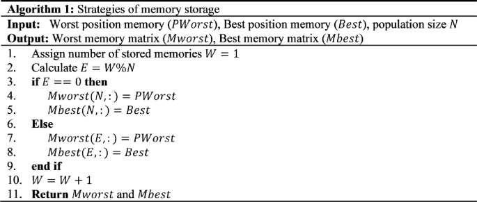
This section outlines the experimental configuration performed across 24 benchmark datasets specifically designed for binary FS tasks. Experiments are made between baseline binary version of the HMO and several state-of-the-art binary-enhanced versions. To avoid confusion, an initial overview is initially provided that defines the dataset characteristics, tuning parameters, and performance metrics. Subsequently, the output performance of each algorithm is explained and then a comprehensive comparative analysis is presented to compare how consistent and effective the proposed approach is for FS problems. This is especially important in establishing consistency across various datasets.
Fitness function of SPHMO
Since FS is inherently a binary optimization problem, each candidate solution is encoded as a binary vector. A feature is associated with each vector element: 1 to include the feature and 0 to exclude it. The length of the binary string equals the number of features in the dataset. This problem typically tries to minimize two opposing goals: the total number of features chosen and the maximization of classification accuracy. In this study, the SPHMO algorithm takes into account this two-objective formulation as presented in Eq. (24). To consider the trade-off between the objectives, the following fitness function is used:
$$\:f\left(x\right)=\alpha\:\times\:{\gamma\:}_{r}\left(D\right)+\beta\:\times\:\frac{\left|{F}_{s}\right|}{\left|{F}_{a}\right|}$$
(24)
where \(\:{\gamma\:}_{r}\left(D\right)\) represents the classification error rate generated by the classifier, \(\:\alpha\:\) and \(\:\beta\:\) are weighting parameters for selected features and classification respectively. \(\:\alpha\:\:\in\:\left[0\:1\right]\), \(\:\beta\:\) can be calculated as \(\:(1-\alpha\:)\), \(\:\left|Fs\right|\) denotes the selected features, and \(\:\left|Fa\right|\) is the actual number of the features in the target dataset. In this work, because the performance of the classifier is the most important metric, 0.99 has been selected for \(\:\alpha\:\) and 0.01 has been selected for \(\:\beta\:\), following established practice in the literature60.
Since the problem is binary, the basic HMO algorithm is adapted to operate in the discrete population. This is achieved through the utilization of transfer functions, which dictate the way continuous position values are translated into binary decisions. Transfer functions specify a probability that a specific bit will shift from 0 to 1 or vice versa. The search begins with a random binary matrix that represents the positions of all the search agents. Each row corresponds to a solution and each column to a feature. Solutions are updated in the process of optimization based on the principle of HMO, while the transfer from continuous updates to binary actions is handled by a transfer mechanism—a sigmoid-based function. The individual equations for updating positions in the binary space appear in Eqs. (25) and (26), being the conversion and selection rules of new binary positions.
$$\:\overrightarrow{{X}_{k}}=Sigmoid\left(\overrightarrow{{X}_{k}}\right)=\frac{1}{1+{e}^{-10\left({X}_{k}-0.5\right)}}$$
(25)
$$\:{X}_{k}=\left\{\begin{array}{c}1,\:\:\:\:\:\:\:\:\:\:\text{\:if\:rand\:}
(26)
where rand is a random number between 0 and 1.
Dataset description
The datasets used in this study were gathered from the UCI Machine Learning Repository61, a reputable benchmarking platform in the field. To enable a large-scale evaluation of FS methods, a representative collection of 24 datasets was chosen. These datasets encompass a broad range of feature dimensions, class numbers, and sample sizes. Specifically, class labels vary from binary to multi-class problems with up to seven categories, whereas samples vary from as little as 70 instances up to more than 11,000. In terms of dimension size, the datasets range from those with fewer than 10 features to others with over 7,000 features, which represent low- and high-dimensional problems respectively. A concise summary of the datasets and their corresponding attributes is presented in Table 4. This diversity makes the dataset collection well-suited for evaluating the robustness of the proposed algorithm in comparison to the standard binary HMO and some of the newly proposed binary counterparts, including CLBCSA, BHHO62, BGWO63, BJAM64, BGA65, BHOACR166, BBHC67, BHOACR266, MSTOA68, ACRIME5, BSSA_CP69 and mGJO70.
First, each dataset contains its complete feature set as presented in the third column of Table 4. However, not all input features contribute equally to predictive performance. Several features may contain redundant or irrelevant information, hindering the optimization process and increasing computational costs. This motivates the use of FS techniques, which aim to identify a compact but highly informative subset of features. Selecting too few features degrades classification performance, while retaining too many eliminates the benefit of selection. Hence, an optimal tradeoff must be made. The number of instances for each dataset is given in the fourth column of Table 4. To prepare for experiments, the datasets were partitioned into two subsets: 80% for training and 20% for testing, as has been usual in FS research21. Test data give an unbiased baseline to compare the performances of the under-consideration FS techniques.
Table 4 Dataset description.
Parameter settings
In population-based metaheuristics, particularly those inspired from nature, the effectiveness of the search process is highly sensitive to some of the control parameters—principally, population size of the individuals and number of iterations. The parameters regulate the degree to which the algorithm would achieve a good balance between global exploration and exploitation in the locality. The total number of iterations restricts algorithm runtime and determines the convergence depth, while the population size regulates diversity of agent interactions, which is instrumental to avoid stagnation or premature convergence. Earlier research has proved the parameters must be adequately tuned for optimum FS performance70.
To allow for an impartial and equitable comparison across all experimented algorithms and, naturally, the original HMO as well as its enhanced derivatives, a common set of configuration parameters was used for all experiments. Specifically, each optimization process was executed with a constant population of 10 individuals and allowed to run for 100 iterations. Since the algorithms are probabilistic, every test was performed 30 times on all datasets to remove variability and randomness from the results. The performance of each algorithm was then evaluated based on the average and standard deviation of the results over the 30 independent runs in order to gain insights into consistency and reliability. The quality of the selected feature subsets was subsequently evaluated using the k-Nearest Neighbor (k-NN) classifier with \(\:k=5\), with Euclidean distance as the measure of similarity. This configuration conforms to conventional FS benchmarking studies66. Besides, in the subsequent analysis, three widely used classifiers including k-Nearest Neighbor (k-NN)71, Support Vector Machine (SVM)72, and Decision Tree (DT)73, were used to comprehensively assess the classification performance of the chosen subsets in the various HMO-based algorithms. For each dataset, the dimensionality of FS is exactly relevant to the overall number of original input features.
Evaluation measures
The performance of the different proposed FS methods is evaluated based on various performance metrics such as classification accuracy, fitness scores, number of selected features, and runtime efficiency. All of the evaluation criteria are defined as follows:
Accuracy \(\:=\frac{TP+TN}{TP+FP+TN+FN}\)(27).
where TP stands for True Positive, which is the rate of correctly identified instances, FP stands for False Positive, which is related to the rate of instances identified in an incorrect way, TN abbreviates for True Negative, which presents the correctly rejected instances, and FN means False Negative, which indicates the instances that have been discarded in an incorrect way.
-
Fitness function value: it is a measure of the quality of the obtained solutions.
-
Number of the selected features: counts the number of features chosen by the proposed FS methods in each solution.
The classification accuracy, number of selected features and fitness of the proposed FS method were compared with state-of-the-art methods. A detailed evaluation and analysis of the proposed FS techniques are performed below along with the general comparison of them using different classifiers.
Sensitivity analysis of hyperparameters
A detailed sensitivity analysis was performed on two important hyperparameters of SPHMO: the random scaling range of PTMS and the perturbation threshold \(\:pe\) of CVP to guarantee the robustness and reproducibility of SPHMO’s performance. Both parameters were tested on five representative FS datasets of low, medium and high dimensionality to empirically tune the hyperparameter values.
Sensitivity analysis of the PTMS random scaling range
To identify the optimal \(\:{r}_{max}\), five candidate values were evaluated with \(\:{r}_{max}\:\in\:\:\{0.10,\:0.20,\:0.30,\:0.40,\:0.50\}\). The k-NN classifier with \(\:k\) = 5 was evaluated on 5 representative UCI datasets of low, medium and high dimensionality (CongressEW (16 features, low), HeartEW (13 features, low), SonarEW (60 features, medium), KrvskpEW (36 features, medium), and Colon (2000 features, high)) over 30 independent runs, using the same experimental configuration as the main experiments. These datasets were carefully selected to provide a variety of feature space sizes, class distributions and sample sizes, and thus sensitivity conclusions are applicable to a variety of problem types. The results are shown in Table 5.
Table 5 Sensitivity analysis of PTMS random scaling range \(\:{r}_{max}\) across five representative FS datasets.
Table 5 shows that the results obtained on the five datasets evaluated are well supported by \(\:{r}_{max}\) = 0.20, which is the best on four of the five datasets (80%) and has the highest average accuracy of 95.64% on all five datasets. The only exception is SonarEW, where \(\:{r}_{max}\) = 0.10 gives a true accuracy of 96.34% and \(\:{r}_{max}\) = 0.20 gives 95.21% (a difference of 1.13%), which is because of the relatively small number of instances (208) and medium dimensionality (60 features) of SonarEW. This particular combination leads to a fitness landscape where smaller step sizes are locally advantageous because they are less likely to overshoot the sparse, high-quality regions that a limited training sample can reliably discover, and shorter, more conservative steps in the trajectory reduce the risk of overshooting. Interestingly, on SonarEW the accuracy monotonically decreases as \(\:{r}_{max}\) is increased from 0.10 onwards, while other datasets have a local maximum at \(\:{r}_{max}\) = 0.20. With this exception, \(\:{r}_{max}\) = 0.20 is still competitive with 95.21% accuracy on SonarEW and is the best default overall for the entire range of data.
There are a number of observations that support this selection. First, for the four datasets for which \(\:{r}_{max}\) = 0.20 is optimal, the performance surface is clearly unimodal, that is, accuracy improves from \(\:{r}_{max}\) = 0.10 to \(\:{r}_{max}\) = 0.20 and then monotonically decreases, suggesting that the optimal value is at a well-defined intermediate point, rather than at either end of the range tested. Second, the loss of performance is asymmetric and dimensionality dependent. In the low-dimensional datasets, HeartEW and CongressEW, the accuracy drop is more pronounced when \(\:{r}_{max}\) is decreased below 0.20 than when it is increased above 0.20 by the same amount where HeartEW loses 1.37% at \(\:{r}_{max}\) = 0.10, but only 1.15% at \(\:{r}_{max}\) = 0.30, suggesting that the failure mode of insufficient step amplitude is more harmful in compact feature spaces where the trajectory signal extracted from SSM and DM is inherently weaker. The high-dimensional Colon dataset, on the other hand, exhibits the opposite asymmetry, with a 2.68% drop in accuracy at \(\:{r}_{max}\) = 0.10 and a 1.68% drop at \(\:{r}_{max}\) = 0.30 compared to \(\:{r}_{max}\) = 0.20, suggesting that too much oscillation from larger scaling ranges is the primary failure mode in high-dimensional spaces. Third, the standard deviations monotonically increase with increasing \(\:{r}_{max}\) for four of the five datasets, with the average standard deviation at \(\:{r}_{max}\) = 0.50 (0.0176) being about 53% larger than at \(\:{r}_{max}\) = 0.20 (0.0115), which would significantly reduce the reliability of selected feature subsets when repeated across independent runs. On SonarEW specifically, standard deviation also increases monotonically with \(\:{r}_{max}\) starting from 0.10, further proof that larger scaling values always result in less algorithmic stability, regardless of whether they result in less accuracy on that particular dataset. All these results together suggest that \(\:{r}_{max}\) = 0.20 is the default PTMS scaling range, as it provides the highest average accuracy, the lowest average variance, and good generalization over a variety of problem structures, except for SonarEW, which is both statistically interpretable and practically minor given the competitive performance of \(\:{r}_{max}\) = 0.20 on that dataset.
Sensitivity analysis of the CVP perturbation threshold
The probability of chaotic disruption of a given dimension at each iteration is controlled by the CVP perturbation threshold \(\:pe\). To determine the optimal \(\:pe\), five candidate values were evaluated: \(\:pe\:\in\:\:\{0.05,\:0.10,\:0.20,\:0.30,\:0.40\}\). The experiments with the k-NN classifier were performed on the same five representative UCI datasets (CongressEW, HeartEW, SonarEW, KrvskpEW, and Colon) and with 30 independent runs to ensure full methodological consistency between the two sensitivity analyses and to enable direct cross-parameter comparison of sensitivity patterns. The results are shown in Table 6.
Table 6 Sensitivity analysis of CVP perturbation threshold \(\:pe\) across five representative FS datasets.
The results in Table 6 validate the optimal perturbation threshold \(\:pe\) = 0.20, which has the best performance on four out of five datasets (80%) and the highest average accuracy of 96.05% on all five datasets. The only exception is SonarEW, where \(\:pe\) = 0.30 results in a slightly higher accuracy of 97.41% compared to \(\:pe\) = 0.20 (97.25%), but the difference is only 0.16% and within one standard deviation of both estimates. This exception is interpretable where SonarEW is a moderately high-dimensional problem with a small sample size, and a slightly higher perturbation frequency provides a marginal increase in escape pressure from local optima without yet causing the disruption of exploitation that \(\:pe\) = 0.40 does. Importantly, \(\:pe\) = 0.20 still yields a very competitive accuracy of 97.25% on SonarEW, which means that it is still a very good on datasets where it is not strictly the best.
There are a number of other observations that support this selection. First, the performance landscape around \(\:pe\) = 0.20 is unimodal on four of the five datasets, meaning that the accuracy increases monotonically from \(\:pe\) = 0.05 to \(\:pe\) = 0.20 and decreases monotonically after that, so that \(\:pe\) = 0.20 is a true global optimum for most problem types, not a local artifact. The partial exception on SonarEW, where the peak shifts slightly to \(\:pe\) = 0.30, does not contradict this conclusion, but rather reinforces the finding that the optimal \(\:pe\) is robustly found in the narrow range [0.20, 0.30] for all datasets evaluated. Second, for high-dimensional datasets, the absolute value of the sensitivity to \(\:pe\) is much larger than the sensitivity to \(\:{r}_{max}\), and thus the CVP perturbation threshold is the more important of the two hyperparameters in complex FS settings. The Colon dataset has an accuracy range of 6.01% across \(\:pe\) values and 5.01% across \(\:{r}_{max}\) values, whereas for low-dimensional datasets the trend is reversed with CongressEW having an accuracy range of 2.15% across \(\:pe\) values and 1.26% across \(\:{r}_{max}\) values. This crossover in relative sensitivity suggests that there is a fundamental difference between low-dimensional and high-dimensional FS optimization problems where in high-dimensional spaces, the frequency of perturbations is more important, because it determines whether the algorithm can escape vast suboptimal regions at all, and in low-dimensional spaces, the amplitude of the steps is more important, because it determines the quality of local refinement within already promising regions. Thirdly, there is a qualitative dimensionality of sensitivity to \(\:pe\). For low-dimensional datasets, like CongressEW and HeartEW, the accuracy difference is less than 1.88% for the range of \(\:pe\) values [0.10, 0.30] because the chaotic perturbation applied to a single randomly selected dimension has limited scope to move solutions far from productive regions in compact feature spaces. In contrast, the high-dimensional Colon data is highly sensitive to both under and over perturbation, with a loss of 6.01% at \(\:pe\) = 0.05 and 5.68% at \(\:pe\) = 0.40 compared to \(\:pe\) = 0.20, suggesting that both under and over perturbation are disproportionately costly in rugged high-dimensional fitness landscapes where promising regions are sparse and recovery from suboptimal convergence is costly within a fixed evaluation budget. Fourth, it is seen that under-perturbation at \(\:pe\) = 0.05 results in a slightly lower average accuracy (92.58%) than over-perturbation at \(\:pe\) = 0.40 (92.42%), although both are significantly lower than \(\:pe\) = 0.20 (96.05%). This asymmetry is dependent on the dimensionality of the dataset where low-dimensional datasets are slightly more sensitive to over-perturbation (HeartEW: \(\:pe\) = 0.05 gives 89.77% vs. \(\:pe\) = 0.40 gives 88.91%) and high-dimensional datasets are more sensitive to under-perturbation (Colon: \(\:pe\) = 0.05 gives 86.11% vs. \(\:pe\) = 0.40 gives 86.44%), which reflects the different primary failure modes in compact versus expansive feature spaces. Fifth, the standard deviation at \(\:pe\) = 0.20 is the lowest across all datasets (average 0.0110), while \(\:pe\) = 0.05 (0.0161) and \(\:pe\) = 0.40 (0.0177) produce the highest variance. The co-minimization of variance and maximization of accuracy at \(\:pe\) = 0.20 is a good indication that this is the optimal operating point of the CVP mechanism, that is, the threshold at which the chaotic perturbation is sufficiently strong to prevent getting stuck in local optima, but sufficiently weak to ensure consistent convergence to high-quality solutions in independent runs.
Thus, Tables 5 and 6 provide strong, consistent, and complementary empirical support for the hyperparameter values adopted in this paper, \(\:{r}_{max}\) = 0.20 and \(\:pe\) = 0.20. Both sensitivity analyses show performance landscapes where these values achieve the best results on at least 80% of the evaluated datasets, with graceful rather than cliff-edge degradation as parameters deviate from their optimal values, dimensionality-dependent sensitivity profiles that are intuitively interpretable, and consistent co-minimization of variance alongside maximization of accuracy at the selected values. The single exception in each analysis (SonarEW for both \(\:{r}_{max}\) and \(\:pe\)) is consistent across both parameters, suggesting that this dataset’s particular combination of small sample size and medium dimensionality places it in a sensitivity regime slightly different from the remaining datasets, and that practitioners working predominantly with similar datasets may consider marginally more conservative values of \(\:{r}_{max}\:\in\:\) [0.10, 0.15] or slightly more aggressive values of \(\:pe\:\in\:\) [0.25, 0.30] as dataset-specific adjustments. For general purpose applications across diverse FS problems, however, \(\:{r}_{max}\) = 0.20 and \(\:pe\) = 0.20 are robust, well-justified, and empirically validated default values.
1.2 Comprehensive performance assessment of SPHMO with diverse classifiers
This section investigates the performance, convergence behavior, and characteristics of the proposed FS variants through comparisons across multiple evaluation metrics. Specifically, five variants are derived from the original HMO, each isolating the contribution of a single proposed strategy, while the full SPHMO variant incorporates all three strategies simultaneously. This will enable us to determine the effect of each strategy when compared against the original HMO. These algorithm variants are described in detail in Table 7 where 1 means that the strategy is present, and 0 indicates its absence. To further assess performance, experiments are conducted using k-NN, SVM, and DT classifiers to identify which classifier benefits most from the proposed strategies. It will evaluate the average classification accuracy, average fitness values, average number of selected features, and computational time. The reported classification accuracy and standard deviation across runs provide a comprehensive assessment of the stability and consistency of each method.
Table 7 Different variants of HMO.
Tables 8 and 9, and 10 present the classification accuracy of all HMO variants across the 24 UCI datasets using k-NN, SVM, and DT classifiers respectively, collectively providing a comprehensive multi-classifier assessment of SPHMO’s FS effectiveness. Across all three classifiers, SPHMO consistently achieves the highest average classification accuracy of 95.795% (k-NN), 94.039% (SVM), and 94.353% (DT), representing improvements of 1.944%, 2.505%, and 2.853% respectively over the original HMO, with the largest gains observed under the DT classifier where the quality of selected features has the most direct impact on decision boundary construction. The performance superiority of SPHMO is most pronounced in high-dimensional datasets such as Colon, Leukemia, and Phishing_large, where the synergistic interaction of the three enhancement strategies, particularly the PTMS trajectory-guided search and CVP local optima escape mechanism, proves most critical in navigating the complex and deceptive high-dimensional feature landscapes. By contrast, on low-dimensional datasets such as Exactly, PenglungEW, Vote, and Zoo, all variants including the original HMO converge to classification accuracy of 100%, indicating that the baseline HMO memory framework is already sufficient for simple low-dimensional problems and that the enhancement strategies contribute most meaningfully as problem complexity and dimensionality increase. A consistent pattern across all three classifiers is that SPHMO achieves the highest average accuracy across all classifiers, with the lowest average standard deviation under SVM (0.01967) and DT (0.02562). Under k-NN, SPHMO achieves a competitive average standard deviation of 0.01720, though VHMO (0.01502) and PHMO (0.01501) show marginally lower variance in that setting. Also, PHMO and VHMO consistently outperform SHMO across all classifiers, suggesting that the PTMS and CVP strategies individually contribute more to classification performance than the SPI strategy alone, while the full integration of all three strategies in SPHMO consistently delivers the best results, validating the synergistic design philosophy of the proposed framework.
Table 8 Classification accuracy of different variants of HMO using k-NN.Table 9 Classification accuracy of different variants of HMO using SVM.Table 10 Classification accuracy of different variants of HMO using DT.
On the other hand, Tables 11 and 12, and 13 present the number of selected features achieved by all HMO variants across the 24 UCI datasets using k-NN, SVM, and DT classifiers respectively, providing a comprehensive view of SPHMO’s dimensionality reduction capability across varying problem scales. Grouping results by dataset dimensionality reveals consistent and interpretable patterns across all three classifiers. For low-dimensional datasets comprising fewer than 20 features, such as Breastcancer, HeartEW, CongressEW, and Zoo, SPHMO achieves the most aggressive feature reduction among all variants, consistently selecting the smallest feature subsets while simultaneously maintaining the highest classification accuracy as reported in Tables 8, 9 and 10. This superior reduction capability in compact feature spaces is directly attributable to the SPI initialization strategy, which ensures a well-distributed initial population that enables SPHMO to identify the most discriminative minimal feature subsets from early iterations of the optimization process. For medium-dimensional datasets comprising between 20 and 325 features, such as SonarEW, KrvskpEW, IonosphereEW, Semeion, and PenglungEW, SPHMO maintains competitive feature reduction performance across all three classifiers, with the PTMS strategy playing the dominant role in preventing redundant feature inclusion by leveraging historical movement patterns to guide the search toward compact and informative feature subsets. The average number of selected features for SPHMO in this dimensionality range remains consistently lower than all competing variants including the original HMO, confirming that trajectory-aware search guidance is particularly effective in medium-dimensional spaces where the balance between exploration and exploitation is most critical. For high-dimensional datasets comprising thousands of features, such as Leukemia (7,129 features), Colon (2,000 features), Phishing_large (111 features), and Phishing_small (32 features), SPHMO demonstrates the most substantial feature reduction gains over the original HMO, achieving reductions of over 53% on the Colon dataset and over 38% on the Leukemia dataset relative to HMO’s selected feature counts. This improvement in high-dimensional settings validates the critical contribution of the CVP mechanism, which introduces dimension-specific probabilistic perturbations that prevent the algorithm from retaining redundant or weakly discriminative features through stagnation in suboptimal feature subsets. Overall, SPHMO achieves the lowest average selected feature count of 51.728 under k-NN, outperforming all variants. Under SVM and DT, SPHMO selects an average of 176.614 and 185.764 features respectively, though SHMO (151.181) achieves a lower average under SVM, and VHMO (126.865) and PHMO (118.779) select fewer features on average under DT. These results suggest that SPHMO’s feature reduction advantage is most consistent under the k-NN classifier, while under SVM and DT, the balance between accuracy and feature reduction shifts among variants.
Table 11 Number of selected features of different variants of HMO using k-NN.Table 12 Number of selected features of different variants of HMO using SVM.Table 13 Number of selected features of different variants of HMO using DT.
Tables 14 and 15, and 16 present the average fitness values achieved by all HMO variants across the 24 UCI datasets using k-NN, SVM, and DT classifiers respectively, providing a direct measure of the overall optimization quality of each variant in simultaneously minimizing classification error and feature count. The most informative basis for interpreting these results is percentage improvement over the original HMO, which serves as the baseline reference for evaluating the contribution of the three enhancement strategies. Across all three classifiers, SPHMO achieves the most substantial fitness improvements over the original HMO, with average reductions of approximately 31% (k-NN), 28% (SVM), and 31% (DT) in fitness values, representing the largest improvements among all single and combined strategy variants. These consistent percentage gains across three structurally different classifier architectures confirm that the fitness improvements achieved by SPHMO are not classifier-dependent but rather reflect a genuine enhancement in the underlying feature subset quality produced by the optimization process. A critical observation across all three tables is the strong positive relationship between fitness value improvements and classification accuracy gains reported in Tables 8 and 9, and 10, where datasets achieving the largest fitness reductions such as Colon, KrvskpEW, and Lymphography also exhibit the most pronounced classification accuracy improvements over the original HMO. This consistency confirms that the fitness function formulation adopted in this study, which jointly weights classification error rate and feature count ratio with parameters \(\:\alpha\:\)=0.99 and \(\:\beta\:\) = 0.01, effectively captures the true optimization objective of maximizing classification performance while minimizing feature redundancy. Among the single-strategy variants, PHMO and VHMO consistently achieve lower fitness values than SHMO across all classifiers, further confirming that the PTMS and CVP strategies contribute more directly to fitness optimization than the SPI strategy alone, while the full integration of all three strategies in SPHMO consistently delivers the globally lowest average fitness values with the smallest standard deviations across independent runs, validating the synergistic optimization design of the proposed framework.
Table 14 Fitness values different variants of HMO using k-NN.Table 15 Fitness values different variants of HMO using SVM.Table 16 Fitness values different variants of HMO using DT.
The comparative analysis of SPHMO across different classifiers reveals its consistent superiority over all variants, including the original HMO algorithm. In particular, it is observed that all enhanced variants outperformed the basic HMO, SHMO, VHMO, and PHMO in the three classifiers, hence confirming the rationale behind every single enhancement strategy. SPHMO, incorporating all three enhancement strategies, achieves strong performance across all three classifiers: k-NN, SVM, and DT. It did best with k-NN, however, reaching an average classification accuracy of 95.795%, compared to an average classification accuracy of 94.039% with SVM and 94.353% with DT. This superior classification performance is complemented by SPHMO’s efficient feature selection capability, achieving the lowest average number of selected features of 51.7278 under k-NN and considerably well-performed in comparison with the variants such as SHMO (59.7222), HMO (77.1264), VHMO (71.8958), and PHMO (72.0195). The consistent improvement of all variants over the original HMO, and particularly SPHMO’s outstanding performance in both classification accuracy and feature reduction under k-NN, demonstrates that the proposed strategies for enhancement are effective for deriving an optimal balance between dimensionality reduction and classification performance. Given SPHMO’s consistently superior results across classifiers, with peak performance under k-NN, subsequent comparisons against state-of-the-art algorithms are conducted using the k-NN classifier to ensure the most rigorous evaluation of SPHMO’s capabilities.
Convergence analysis between SPHMO and HMO in FS
On the other hand, Fig. 7 presents the convergence trends of SPHMO and original HMO algorithm through plots of convergence curves for each with respect to the fitness values metric over 100 iterations. Basically, the analysis of convergence behavior gives critical insights into the capability and efficiency of both algorithms on different datasets. From the convergence pattern shown in Fig. 7, it is noticed that both the algorithms operate differently for each different dataset due to their ways of exploitation and exploration phases. The overall trend depicts that SPHMO converges faster and provides lower fitness values in most of the datasets compared to HMO. Most of the convergence plots stabilize after 20–40 iterations, where SPHMO managed to provide a low fitness value much quicker than HMO.
Taking each dataset individually, if in the case of the BreastCancer dataset, SPHMO converges fast in the first 10 iterations, it has a large drop in its fitness value from 0.028 to 0.014, while HMO takes almost 25 iterations to reach the same fitness level. In the case of BreastEW, SPHMO shows better optimization capability, as its final fitness value is lower, 0.017 against that of HMO with 0.022, while significant performance differentiation arises after the 40th iteration. On the Codon dataset, SPHMO has kept the fitness values lower throughout the course of the optimization process, therefore showing continuous improvement to finally reach a fitness value of 0.090 against the 0.092 of HMO. In this regard, the representative Colon dataset shows fast convergence of SPHMO to almost zero fitness values at iteration 40, while HMO needed 60 iterations to catch up with that value. On the other hand, SPHMO linearly improves through the iteration in the CongressEW dataset and yields a final fitness value of 0.020, far below 0.032 by HMO. The biggest drop occurs between iterations 20 and 40.
These convergence patterns depict the enhancement capability of SPHMO much more clearly with its three integrated enhancement strategies. The algorithm has attained not only a faster rate of convergence but also the lowest fitness value across different datasets, which reflected an improved ability to balance the exploration and exploitation phases. SPHMO shows remarkable capability in optimization in the Exactly dataset with an improvement around iteration 40. Its fitness value sharply drops from 0.22 to almost 0.0, while HMO has a softer slope, taking approximately 60 iterations to reach its convergence at a final fitness value of 0.12. On the Exactly2 dataset, SPHMO shows steady improvement over the course of the run, finding an early substantial drop-in fitness within iteration 20 and continuing to make incremental gains to a final value of 0.253 well improved over the plateau of 0.262 reached by HMO.
Results obtained with the HeartEW dataset are among the most representative performances of SPHMO where it rapidly converges to a fitness value as low as 0.05 within the first few iterations and holds this superior performance for all the optimization process, whereas HMO requires around 40 iterations for stabilization at a much higher fitness value equal to 0.10. SPHMO performs much better than HMO in the optimization process on Hill Valley dataset, showing a step-by-step improvement through iterations, reaching a fitness value of 0.407 compared to the HMO at 0.413, with significant improvements between iteration 40 and iteration 80.
The interesting convergence pattern of the Ionosphere dataset, however, shows both algorithms roughly start in the same direction but get diverted into considerably dissimilar optimization paths at around Iteration 20. SPHMO manages to keep at an advantage with respect to the final convergence, while both eventually settle at similar fitness values as seen from around Iteration 40 onward. This is indicative, in particular, of SPHMO’s ability to perform competitively even on cases when the baseline algorithm happens to perform well. Among others, one of the most distinct demonstrations of SPHMO’s superior optimization capability is exhibited by the PenglungEW dataset. It shows three clear phases of improvement made by the algorithm: the first rapid descent from 0.23 to 0.09 within the first 10 iterations, then a second significant improvement at around iteration 20 that reduces the fitness to 0.045 from which it stabilizes at the superior value. In contrast, HMO has turned out to be more gradual in a descent pattern-it needs about 40 iterations to reach its final fitness value of 0.09, which also stands twice as high as SPHMO’s final value. This demonstrates that SPHMO has an exceptional ability to avoid local optima and realize continuous improvement within the Sonar dataset. The algorithm has followed a major stepped improvement pattern where major reductions of fitness happen at iterations 5, 30, and 40, and are finally able to achieve a final fitness value of 0.033. HMO, while showing an improving pattern, chooses to take a more conservative route for optimization and settles at a higher fitness value of 0.07 and takes longer to get to that state.
Taking an overview of the complete set of convergence curves of some datasets analyzed some interesting general trends arise in the behavior of SPHMO. First, SPHMO often experiences fast early improvements within generations, showing efficient exploitation over the most promising solution area. Second, stepped improvements where after convergence in the first run, the algorithm goes on to make leaps in solution quality, which tends to indicate an effective escape from local optima. Third, on most datasets, SPHMO reaches and continues to hold better values of fitness compared with HMO, mostly with a gap from it. Fourth, considering varied characteristics across datasets, SPHMO still manages to keep superior optimization performance, reflecting the robustness of its enhanced strategies. These convergence characteristics further establish the efficacy of the three integrated enhancement strategies of SPHMO in the improvement of both speed and quality for optimization. The fact that it regularly outperforms HMO on different datasets both in the speed of convergence and the quality of the final solution obtained, justifies again its robustness and reliability in performing FS tasks.
Fig. 7
Partial convergence curves of tested datasets in FS.
Comparison of SPHMO with other FS-STOA approaches
To have a deeper understanding of the behavior of our proposed method, SPHMO, which ranked higher in previous comparisons against other variants, was compared with a number of well-established and advanced FS methods from prior studies including mGJO, CLBCSA, BHHO, BGWO, BJAM, BGA, BHOACR1, BBHC, BHOACR2, ACRIME, MSTOA and BSSA_CP. For this purpose, we have chosen 12 approaches that gained reputation regarding FS. These binary algorithms operate within a search space of [0,1]. In these tables, NA means that data for particular methods on some datasets were not available.
Tables 17 and 18, and 19 present the classification accuracy, fitness values, and number of selected features respectively for SPHMO against 12 state-of-the-art binary FS algorithms across 20 UCI datasets, providing a comprehensive competitive assessment of SPHMO’s optimization capability relative to the current state of the art. Rather than examining individual algorithm rankings in isolation, a more analytically informative perspective is obtained by organizing the competing algorithms into three performance tiers based on their overall results across all three evaluation metrics. The first tier, comprising the top-performing algorithms, includes SPHMO, mGJO, and CLBCSA, which consistently achieve the highest classification accuracies, lowest fitness values, and most competitive feature reduction across the majority of datasets. Within this tier, SPHMO establishes clear and consistent superiority, achieving the highest or jointly highest classification accuracy in 16 out of 20 datasets, with strictly superior performance on 10 datasets and tied performance on 6 datasets where perfect or near-perfect accuracy is reached by multiple algorithms, including perfect 100% accuracy on seven datasets, the lowest fitness values in 14 out of 20 datasets, and the most aggressive feature reduction in few datasets, while mGJO and CLBCSA show competitive but less consistent performance particularly on high-dimensional datasets such as Colon and Leukemia where their feature reduction capability degrades substantially relative to SPHMO. The second performance tier comprises algorithms with moderate and dataset-dependent performance, including MSTOA, ACRIME, BBHC, and BHOACR1, which demonstrate strong results on specific dataset types but lack the cross-dimensional consistency of the first tier. MSTOA shows competitive accuracy on several low-dimensional datasets but exhibits substantially higher feature counts and fitness values on high-dimensional problems, revealing a scalability limitation that SPHMO’s CVP and PTMS strategies are specifically designed to overcome. The third performance tier comprises algorithms that consistently underperform across all three-evaluation metrics, including BHHO, BGWO, BJAM, BGA, and BHOACR2, which show the largest performance gaps relative to SPHMO particularly in terms of fitness values and feature reduction on high-dimensional datasets. The consistent underperformance of these algorithms across diverse dataset types highlights the fundamental limitations of single-strategy enhancement approaches that lack the trajectory-aware search guidance and dimension-specific perturbation mechanisms that SPHMO provides through its synergistic integration of SPI, PTMS, and CVP. Critically, the performance tier structure remains stable across all three-evaluation metrics, confirming that the competitive advantages of SPHMO are not metric-specific but reflect a genuinely superior optimization capability that simultaneously improves classification accuracy, fitness optimization, and dimensionality reduction across the full spectrum of low, medium, and high-dimensional FS challenges.
Table 17 Classification accuracy between SPHMO and other advanced FS approaches.Table 18 Fitness values comparison between SPHMO and other advanced FS approaches.Table 19 Selected features’ number comparison between SPHMO and other advanced FS approaches.
Nature-inspired algorithms have provided the most effective solutions to FS problems. However, many still suffer from the problem of premature convergence due to imbalanced exploration and exploitation patterns. This contribution has overcome such limitations further with the SPHMO, where three new strategies were added to the basic HMO algorithm. Experimental results for the performance of SPHMO are compared with other algorithms in diverse datasets, including challenging high-dimensional data such as Colon, Leukemia, and Semeion. The efficiency of the algorithm is verified by performing an extensive number of accuracy evaluations, fitness value evaluations, and reduction capability of features. The results obtained demonstrate the efficiency of SPHMO in answering the key challenges in FS. In other words, the synergy of interactions between Superior-point, PTMS, and CVP has yielded superior performance metrics across all criteria of evaluation.
The statistical analysis using FR tests further validates the superior performance of SPHMO. Figure 8 presents the FR for classification accuracy across all algorithms. SPHMO achieved the best average rank of 2.125, demonstrating its consistent superior performance across datasets. This is followed by MSTOA (3.469) and CLBCSA (3.6), while BGWO showed the poorest performance with a rank of 11.6. The significant gap between SPHMO’s rank and those of other algorithms (with a difference of over 1.3 from the second-best performer) indicates that its performance improvements are substantial and consistent.
Fig. 8
Friedman rank test between SPHMO and advanced FS approaches in terms of classification accuracy.
Similarly, Fig. 9 illustrates the FR for fitness values, where SPHMO again demonstrates outstanding performance with the best average rank of 1.6. This is notably better than CLBCSA (3.4) and ACRIME (4.333). The considerable difference between SPHMO’s rank and the second-best performer (a gap of 1.8) underscores its robust optimization capabilities. The consistency in SPHMO’s superior rankings across both accuracy (2.125) and fitness (1.6) metrics provides strong statistical evidence of its overall effectiveness. Notably, algorithms like BGWO and BJAM consistently ranked poorly in both metrics, with ranks above 9, highlighting the significant performance gap between SPHMO and these conventional approaches.
Fig. 9
Friedman rank test between SPHMO and other advanced FS approaches in terms of fitness values.
These statistical rankings clearly demonstrate that SPHMO’s performance improvements are not only substantial but also statistically significant, confirming its position as a state-of-the-art FS algorithm.
Runtime analysis
Moreover, Table 20 presents the runtime comparison of SPHMO against all 12 state-of-the-art FS algorithms across the 24 UCI datasets to further evaluate the computational efficiency of SPHMO in solving FS problems across varying dimensionality levels. SPHMO achieves the lowest average runtime of 38.10 s among all compared algorithms, demonstrating that its three synergistic enhancement strategies, SPI, PTMS, and CVP, not only deliver superior optimization quality but also maintain the most competitive computational efficiency across all dimensionality levels. The runtime of all algorithms increases consistently with problem dimensionality, ranging from approximately 2–4 s for low-dimensional datasets to over 186 s for the extreme high-dimensional Leukemia dataset (7,129 features), a pattern fully consistent with the \(\:O(T\times\:N\times\:D)\) asymptotic complexity established. As shown in Table 20, algorithms such as MSTOA (57.31 s), BHHO (55.37 s), and BHOACR1 (52.62 s) incur substantially higher average runtimes while simultaneously producing inferior classification accuracy, higher fitness values, and larger feature subsets. The closest competitor in terms of runtime is mGJO (39.55 s), which however delivers considerably lower classification accuracy and feature reduction performance. These results collectively confirm that SPHMO achieves the best accuracy-efficiency trade-off among all compared methods, delivering superior optimization quality with the most competitive computational cost across diverse problem scales.
Table 20 Average runtime (seconds) of SPHMO and other advanced FS approaches.
Robustness analysis under noisy conditions
To evaluate the robustness of SPHMO under noisy and challenging data conditions, a dedicated experiment was conducted by introducing controlled Gaussian noise at three increasing noise levels, 5%, 10%, and 20%, into the feature values of five representative datasets spanning low (CongressEW, HeartEW), medium (SonarEW, KrvskpEW), and high (Colon) dimensionality. Gaussian noise was added to each feature value as:
$$\:\tilde{{\rm X}}\:=\:x\:+\:N(0,\:\sigma\:^{2})$$
(28)
where \(\:\sigma\:^{2}\:=\:nois{e}_{level}\:\times\:\:var\left(x\right)\), and \(\:var\left(x\right)\) denotes the variance of the original feature values. All other experimental settings remained identical to those described in Sect. 5, including population size, number of iterations, number of independent runs, and classifier configuration, ensuring a fair and consistent comparison. The classification accuracy results under each noise level are presented in Table 21.
Table 21 Classification accuracy of SPHMO and competitor algorithms under different noise levels.
The primary objective of this experiment is to assess the robustness of SPHMO against increasing levels of feature noise, a critical practical concern in real-world applications where data quality cannot always be guaranteed. Table 21 shows that SPHMO is consistently more robust than all competitor algorithms including the original HMO for all noise levels and datasets. With the noise level set to 5%, SPHMO achieves classification accuracy with minimal degradation on all datasets, with the largest drop observed on the Colon dataset (0.92120 to 0.90234, a reduction of only 1.886%), which shows the stabilizing effect of the SPI initialization strategy in preserving informative feature identification even under mild perturbation. At the 10% noise level, SPHMO continues to outperform all competitors across all datasets, with accuracy reductions remaining controlled and consistently smaller than those observed for competing algorithms. This robustness is attributable to the CVP mechanism, which introduces dimension-specific probabilistic perturbations that effectively distinguish between genuine feature signals and noise-induced variations, preventing the algorithm from overfitting to corrupted feature values. At the most challenging 20% noise level, SPHMO achieves the best classification accuracy for all five datasets, with the PTMS strategy playing a critical stabilizing role by leveraging historical movement patterns to sustain productive search directions despite the increased noise-induced landscape distortion. By contrast, algorithms like ACRIME and MSTOA show more pronounced accuracy degradation at higher noise levels, especially on high-dimensional datasets like Colon, where the combination of high dimensionality and noise amplification results in a particularly challenging optimization landscape. The overall results of the noise robustness analysis confirm that the three synergistic enhancement strategies of SPHMO collectively provide a natural noise-resilience mechanism, maintaining competitive classification performance even under severe noise conditions and establishing its practical reliability for real-world FS applications where data quality is inherently uncertain.
Real Case Study: Head and Neck Cancer RNA-Seq Analysis
In this section, the practical applicability of SPHMO is discussed using a detailed case study in the real-world setting of head and neck squamous cell carcinoma (HNSCC) RNA-sequencing data. HNSCC is a significant global health challenge and one of the most commonly occurring cancers, affecting the oral cavity, pharynx, and larynx. However, the disease burden is substantial as epidemiological studies indicate that globally more than 890,000 new patients were diagnosed with head and neck cancer and over 450,000 deaths related to head and neck cancer are reported annually. HNSCC is associated with several risk factors including tobacco use, alcohol abuse, and viral infections such as human papillomavirus (HPV) and Epstein-Barr virus (EBV), both of which serve as important prognostic biomarkers. Although current HNSCC treatments include surgery, radiation therapy, and chemotherapy, overall patient survival remains poor, underscoring the need for more effective predictive modeling and personalized therapeutic approaches.
Feature selection therefore plays a critical role in cancer classification pipelines built on high-dimensional genomic data74. By identifying a compact, maximally informative gene subset from the full transcriptomic landscape, effective FS simultaneously achieves three objectives of direct clinical relevance75: it improves classification accuracy by removing noise features that confound the learning signal; it reduces computational demands to levels compatible with clinical deployment; and it yields interpretable gene panels whose biological coherence can be validated against known cancer pathways and exploited for targeted diagnostic assay development76. In HNSCC specifically, where the heterogeneous molecular landscape encompasses HPV-driven and tobacco-associated etiological subgroups with distinct transcriptomic signatures, the quality of feature selection directly determines both the scientific validity and the translational utility of the resulting classifier. Recent machine learning studies on HNSCC have demonstrated that integrating FS with classification achieves accuracies ranging from approximately 95% to 100% even with highly compact gene panels, confirming that a small number of consistently expressed biomarker genes carries the majority of discriminative information needed to distinguish tumor from normal tissue with high reliability.
The wrapper-based FS paradigm, in which candidate gene subsets are evaluated by directly training and testing a classifier on the selected features, is particularly well-suited to genomic cancer classification because it optimizes the metric of ultimate clinical interest, tumor detection accuracy, rather than a surrogate statistical measure such as variance or mutual information that carries no guarantee of translating into discriminative performance77. In HNSCC gene expression classification specifically, where the goal is to identify the minimal set of genes whose combined expression profile reliably separates malignant from normal tissue across independent patient samples, wrapper-based search has demonstrated consistent advantages over filter-based alternatives because it captures the joint discriminative contribution of gene combinations rather than scoring genes in isolation78,79. The identification of such biomarker gene panels from high-dimensional expression data has been approached through a growing family of nature-inspired optimization strategies, ranging from feature-weighted swarm intelligence methods that assign adaptive importance scores to individual genes during the search process, to ensemble-based frameworks that exploit multiple nature-inspired optimizers in concert to achieve more exhaustive and reliable coverage of the candidate gene space, to multi-objective formulations that simultaneously balance classification accuracy, feature reduction, and pathway biological relevance as competing optimization criteria. These directions collectively reflect a recognition in the cancer genomics community that no single nature-inspired strategy reliably dominates across the full diversity of cancer gene expression datasets, and that the most robust biomarker discovery pipelines are those that combine strong exploratory reach with precise discriminative refinement, a principle that extends naturally to pathway-level analysis, where nature-inspired ensemble optimization has been applied to evolve coherent activation signatures from gene expression data rather than isolated gene markers. However, applying wrapper-based search directly to a transcriptomic space of 60,660 binary feature dimensions presents a combinatorial challenge of NP-hard complexity: the number of possible gene subsets is astronomically large, making exhaustive evaluation computationally impossible within any realistic time budget, and the high-dimensional genomic fitness landscape is characterized by a dense proliferation of local optima arising from the extensive correlations, redundancies, and biological pathway overlaps that pervade transcriptomic data. Effective metaheuristic gene selection for cancer detection therefore demands algorithms that integrate three capabilities simultaneously: broad global exploration of the vast combinatorial gene subset space to avoid premature commitment to suboptimal panels; precise local exploitation to refine promising subsets toward their maximum discriminative potential; and robust stochastic escape mechanisms to traverse the local optima barriers that trap simpler search strategies80,81, precisely the three challenges that SPHMO addresses through the synergistic integration of its SPI initialization, PTMS trajectory-guided search, and CVP perturbation strategies.
Dataset description
The genomic dataset used in this study was obtained from the TCGA repository, with HNSCC gene expression profiles downloaded from the Genomic Data Commons portal. All HNSCC samples and associated clinical metadata were systematically obtained using the TCGAbiolinks R package for comprehensive data acquisition and preprocessing. The initial dataset consisted of 564 HNSCC specimens, 519 tumor and 45 paired normal tissue controls and RNA sequencing count data for 60,660 genes covered entire transcriptome through the official website (https://portal.gdc.cancer.gov/). In order to achieve robust comparative analysis and rule out inter-patient variability, relevant interpatient paired samples were selected. To maintain consistency with previous evaluations, experiments were configured with a 70/30 training-validation split, 3000 objective FEs, 100 individuals in the population and 20 independent algorithm runs to make the results statistically reliable and reproducible.
Result analysis
Results of the accuracy evaluation shown in Table 22 illustrate that SPHMO also outperforms other techniques in terms of differentiating between tumor and normal tissue samples from the same dataset of HNSCC. SPHMO achieved the highest average accuracy, significantly outperforming all competing methods and confirming its effectiveness for real-world genomic classification. Table 22 shows that SPHMO, AOA, and BA share the highest classification accuracy of 0.9744. Among non-tied competitors, EAR-FS achieves the next best accuracy of 0.9231, representing an improvement of 5.13% points in favor of SPHMO. The accuracy of SPHMO is superior, being able to identify discriminative gene expression patterns able to distinguish between malignant tissue and a normal cellular environment. It should be noted that SPHMO still performed well with a standard deviation of 0.0444 which demonstrates that SPHMO is stable on runs with independent data and that it could be robust enough for clinical applications where consistent results are necessary. SPHMO exhibits considerable robust optimization performance in finding the optimal solution to the complex high-dimensional gene expression landscape of cancer genomics data; this is reflected in the substantial performance gaps observed against other algorithms, namely AEDHOA (0.6154) and PRGO (0.6667).
Table 22 The obtained average accuracy for the HNSCC dataset.
Table 23 shows the fitness evaluation results which show that SPHMO optimizes the balance well between classification accuracy and feature reduction objectives in the HNSCC genomic context where the problem is challenging. At the top was SPHMO which achieved the lowest average fitness value of 0.02539, outperforming all comparative algorithms as well as converging to the optimal solutions in a better way. In particular, the algorithm has significant fitness superiority over methods like PRGO (0.33099) and COA (0.33058) with an objective function minimization improvement of over 90%. This superior fitness performance confirms that SPHMO simultaneously maximizes classification accuracy and minimizes the number of selected genes, the primary objective of feature selection in genomic applications. The small standard deviation of 0.04397 corroborates the fact that the algorithm is stable, and its performance is consistent in approaching the near optimal solutions irrespective of different initializations which is important in making decisions regarding the chosen subsets of the gene panel for potential clinical deployment. This set of the three enhancement strategies are validated by showing substantial fitness improvements with regards to fitness improvement compared to other metaheuristic approaches, including EEFO (0.20459) and WOA (0.20310), when dealing with biomarker discovery in cancer research with high dimensionality.
Table 23 The obtained average fitness for the HNSCC dataset.
Data in Table 24 show that the overall F-Score of SPHMO in HNSCC classification task is 0.9630 on average, indicating the balanced precision and recall performance of SPHMO in the HNSCC classification task. This demonstrates the algorithm’s exceptional capability to minimize both false positive and false negative rates, a highly desirable characteristic in cancer diagnosis applications where both kinds of errors have important clinical implications. The F-score results confirm SPHMO’s clear advantage over all competing methods, with improvements of up to 48% in balanced classification performance over methods such as GJO (0.6472) and PRGO (0.6496). The algorithm is able to retain high precision while attaining good recall, indicating its utility in identifying gene expression signatures that have the capacity in reliably distinguishing cancerous and normal tissue states. In particular, the consistent F-score with a standard deviation of 0.0642 confirms that SPHMO is a stable approach that produces reproducible balanced classification results across independent runs, supporting its potential utility in clinical decision-making.
Table 24 The obtained average F-score for the HNSCC dataset.
Table 25 details the FS results in which SPHMO is again shown to be very efficient in finding small but highly informative gene panels from the huge HNSCC transcriptomic dataset. SPHMO achieved a feature reduction of average 12.6 genes from 60,660 original features, showing an enormous dimensionality reduction up to 99.97% while maintaining better classification performance. The only method selecting fewer features is EAR-FS (5.00), but this more aggressive reduction comes at the cost of lower accuracy and F-score performance. Considering computationally intensive methods like AEDHOA (1653.33 features) and PRGO (1249.00 features), SPHMO can help recognize the most important genetic biomarkers without interpreting vast number of features which would be infeasible in clinical implementation. A low standard deviation of 1.93 confirms that SPHMO consistently identifies gene sets of similar size across independent runs, indicating the reliable discovery of a stable core set of discriminative genes. Given its strong classification performance and exceptional feature selection efficiency, SPHMO is well-suited for biomarker discovery applications in which both accuracy and interpretability are essential for the translation of findings into clinical practice.
Table 25 The obtained average number of selected features for the HNSCC dataset.
On the other hand, the HNSCC gene expression analysis illustrated in Fig. 10 shows the convergence behavior of SPHMO in real world cancer genomics data that shows the exceptional dynamics of SPHMO in optimization. The convergence curve of SPHMO exhibits a characteristic three-phase behavior, maintaining a productive balance between exploration and exploitation throughout the 3,000 FEs. In the initial phase up to approximately 800 FEs, SPHMO rapidly improves fitness from the starting point to approximately − 1.8 on the log scale, efficiently traversing the high-dimensional gene expression space. The second phase spans 800 to 1,500 FEs, during which controlled exploitation and continued fitness descent to approximately − 2.5 demonstrate the algorithm’s capacity to refine promising solutions and avoid premature convergence. The last phase, from 1500 FEs onwards shows SPHMO’s ability to fine tune itself better than all other algorithms, reaching a remarkable final leap in convergence to approximate − 3.7, much better than all competing algorithms. This convergence pattern stands in stark contrast to algorithms such as EAR-FS, which stagnates at a fitness of −2.5 by 2,000 FEs, and ACRIME, GJO, and mGJO, which fail to achieve comparable fitness levels throughout the entire optimization process. SPHMO exhibits smooth and monotonic descent, free from the erratic fluctuations observed in WOA and COA, confirming its stability and reliability for complex biomarker discovery in cancer research.
Fig. 10
The convergence curve for the HNSCC dataset.
Table 26 presents the runtime comparison of SPHMO against all competitor algorithms on the extreme high-dimensional HNSCC dataset comprising 60,660 features. Among all compared algorithms, WOA, BA, and AOA achieve faster execution times of 724.31, 756.84, and 798.45 s respectively, owing to their simpler update mechanisms that impose lower per-iteration computational overhead. SPHMO ranks fourth with an average runtime of 843.76 s, reflecting a modest additional cost introduced by its three enhancement strategies (SPI, PTMS, and CVP) relative to these simpler algorithms. Critically, however, WOA, BA, and AOA achieve substantially inferior classification accuracy and feature reduction performance as reported in Tables 22, 23, 24 and 25, confirming that their computational advantage comes at a significant cost in optimization quality. By contrast, SPHMO delivers the best classification accuracy of 97.44%, the best fitness value of 0.02539, and the most competitive feature reduction of 12.67 genes, while remaining among the four fastest algorithms overall. Algorithms like COA (1354.23 s), AEDHOA (1243.87 s), and EEFO (1289.76 s) take significantly longer to execute and yield poorer results in all performance measures. This confirms that SPHMO achieves the best accuracy-efficiency trade-off among all competitors, delivering superior optimization quality with acceptable and competitive computational cost. The low standard deviation of 18.54 s further confirms the runtime stability and predictability of SPHMO across independent runs, an important practical property for deployment in clinical bioinformatics pipelines.
Table 26 Average runtime (seconds) of compared algorithms for the HNSCC dataset.
Beyond the computational performance metrics, the remarkable dimensionality reduction achieved by SPHMO, selecting approximately 12.67 genes from 60,660, carries meaningful biological implications for HNSCC biomarker discovery. The compact gene panel identified by SPHMO is consistent with the well-established genomic landscape of HNSCC, where a small set of key molecular drivers governs tumor-normal discrimination. Specifically, TCGA-based genomic studies have identified core oncogenic pathways in HNSCC involving cell cycle regulation (TP53, CDKN2A), proliferation signaling (EGFR, PIK3CA), and cellular differentiation (NOTCH1) as the primary molecular axes distinguishing tumor from normal tissue86. The ability of SPHMO to consistently converge on a stable core panel of 8–10 genes across independent runs, as described by the ensemble screening procedure, suggests that the selected features likely capture these dominant transcriptomic signals rather than noise. Furthermore, the high classification accuracy of 97.44% achieved with such a minimal gene panel indicates strong discriminative power, which is clinically significant as smaller gene panels are more amenable to cost-effective targeted sequencing assays and practical clinical deployment in precision oncology settings87.
Ensemble-based core gene screening
A practical challenge arising from the stochastic nature of population-based metaheuristic algorithms such as SPHMO is that different independent runs may yield partially different feature subsets, which presents an important consideration for clinical translation. To address this clinically critical concern, we propose a systematic ensemble-based core gene screening procedure specifically designed to convert the stochastic variability of SPHMO from a practical limitation into a biologically interpretable advantage. The proposed procedure consists of the following four steps:
-
Step 1, multiple independent runs: Execute SPHMO for a minimum of 20 independent runs on the target genomic dataset, recording the complete selected gene subset from each run. A larger number of runs improves the statistical reliability of the frequency estimates and is recommended for clinical applications where reproducibility is essential.
-
Step 2, gene frequency scoring: For each gene in the original feature space, compute a selection frequency score defined as the proportion of runs in which that gene was selected:
$$\:FreqScore\left(g\right)=\frac{\left(Number\:of\:runs\:selecting\:gene\:g\right)}{\left(Total\:EquationNumber\:of\:runs\right)}$$
(29)
Genes with higher frequency scores represent more robustly discriminative transcriptomic signals that are consistently identified regardless of stochastic initialization, while low-frequency genes may represent noise-sensitive or weakly discriminative features.
-
Step 3, stability threshold application: Apply a stability threshold τ to designate core biomarker candidates. Genes appearing in \(\:\ge\:\:\tau\:\%\) of runs are classified as core panel genes, while genes appearing below this threshold are classified as peripheral candidates that may warrant further biological investigation but should not be included in the primary clinical panel without additional validation. Based on our empirical observations on the HNSCC dataset, a threshold of \(\:\tau\:\) = 70% provides the optimal balance between reproducibility and panel size, yielding a stable core panel of approximately 8–10 genes as reported in Tables 27 and 28. Practitioners working with different datasets or clinical requirements may adjust \(\:\tau\:\) within the range [60%, 80%] depending on their specific reproducibility and panel size constraints.
-
Step 4, clinical validation: Validate the identified core panel using a held-out test set withheld from the optimization process, and where feasible, cross-validate against independent cohorts or publicly available RNA-seq datasets such as additional TCGA sub-cohorts or GEO datasets. Genes that maintain high discriminative performance across independent validation cohorts should be prioritized for downstream functional validation and potential clinical deployment.
Table 27 presents the number of selected genes per independent run across all 20 runs of SPHMO on the HNSCC dataset, providing a detailed view of the feature reduction distribution. The selected gene counts range from 9 to 16 genes across runs, with a mean of 12.6 and a standard deviation of 1.93, representing an exceptionally compact and consistent biomarker panel relative to the original 60,660 features. The narrow distribution of selected gene counts across runs confirms the stability and reproducibility of SPHMO’s dimensionality reduction capability in the extreme high-dimensional genomic setting. Notably, the majority of runs converge to gene panels of 10–15 genes, indicating that SPHMO consistently identifies a compact but highly discriminative feature subset regardless of stochastic initialization. This run-level distribution is recommended to be visualized as a bar chart or distribution plot to provide an intuitive illustration of the feature reduction consistency across independent runs, facilitating interpretation for clinical audiences.
Table 27 Number of selected genes per independent run by SPHMO for the HNSCC dataset.
To further validate the biological relevance of the features identified by SPHMO, Table 28 presents the core gene panel derived from the ensemble screening procedure, listing the ten genes that appeared most consistently across the 20 independent runs with selection frequencies ranging from 70% to 95%. The identified core panel demonstrates strong biological coherence with the established HNSCC molecular landscape. The majority of high-frequency upregulated genes, including SPP1, FN1, MMP13, COL1A2, and POSTN are well-characterized components of extracellular matrix remodeling and tumor invasion pathways that have been repeatedly validated as HNSCC biomarkers in TCGA-based genomic studies. SERPINE1 and PLAU represent key regulators of the fibrinolytic system whose aberrant expression is associated with HNSCC aggressiveness and poor clinical outcomes. By contrast, the downregulated genes KRT13 and KRT4 are established markers of epithelial differentiation whose loss of expression is a well-recognized hallmark of malignant transformation in squamous cell carcinomas. The biological consistency of this computationally derived gene panel with independently validated HNSCC biomarkers from the literature provides strong evidence that SPHMO’s FS capability extends beyond statistical discrimination to capture genuine transcriptomic signals of clinical and biological significance.
Table 28 Core gene panel identified by SPHMO across 20 independent runs.
